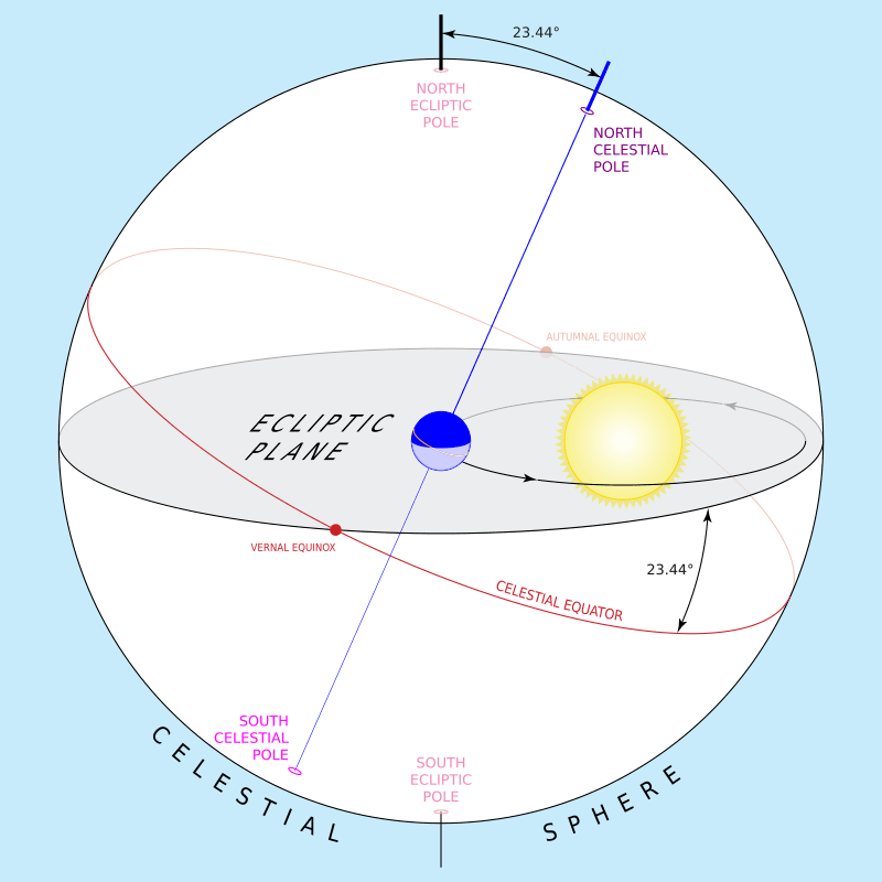

The polar or rotational axis of the planet Earth is tilted at an angle of approximately 23.44 degrees to the plane of the Earth’s orbit around the Sun. The tilt is called the obliquity and the plane of the Earth’s orbit is called the ecliptic, because that is where we see eclipses. The graphic above illustrates this obliquity to the ecliptic plane as the Earth travels in orbit around the Sun, which is the predominant cause of annual seasons on Earth.
The plane of Earth’s orbit projected in all directions forms the reference plane known as the ecliptic. Here, it is shown projected outward (gray) to the celestial sphere, along with Earth’s equator and rotational polar axis (green). The plane of the ecliptic intersects the celestial sphere along a great circle (black), the same circle on which the Sun seems to move as Earth orbits it. The intersections of the ecliptic and the equator on the celestial sphere are the equinoxes (red), where the Sun seems to cross the celestial equator. Wikipedia1
In ancient times astronomers calculated and tabulated ephemerides (plural of ephemeris, meaning ‘diary’ from Ancient Greek ἐφημερίς (ephēmerís)), a book with tables that gives the trajectory of naturally occurring astronomical objects in the sky, i.e., their positions over time.
Historically, positions were given as printed tables of values, given at regular intervals of date and time. The calculation of these tables was one of the first applications of mechanical computers. Modern ephemerides are often provided in electronic form. However, printed ephemerides are still produced, as they are useful when computational devices are not available.2
For scientific uses, a modern planetary ephemeris comprises software that generates positions of planets and often of their satellites, asteroids, or comets, at virtually any time desired by the user.
After introduction of electronic computers in the 1950s it became feasible to use numerical integration to compute ephemerides. The Jet Propulsion Laboratory Development Ephemeris is a prime example. Conventional so-called analytical ephemerides that utilize series expansions for the coordinates have also been developed, but of much increased size and accuracy as compared to the past, by making use of computers to manage the tens of thousands of terms. Ephemeride Lunaire Parisienne and VSOP are examples.
Typically, such ephemerides cover several centuries, past and future; the future ones can be covered because the field of celestial mechanics has developed several accurate theories. Nevertheless, there are secular phenomena which cannot adequately be considered by ephemerides. The greatest uncertainties in the positions of planets are caused by the perturbations of numerous asteroids, most of whose masses and orbits are poorly known, rendering their effect uncertain. Reflecting the continuing influx of new data and observations, NASA’s Jet Propulsion Laboratory (JPL) has revised its published ephemerides nearly every year since 1981.
Newcomb’s Formula
Until 1983 the obliquity (ε) of the ecliptic for any date was calculated from the work of Simon Newcomb, who analyzed positions of the planets until about 1895. It is a formula named after Newcomb and takes a polynomial form as a function of universal time from a reference year.
Newcomb’s formula is an empirically derived polynomial representation of the effect of the combined gravitational pull of the Sun, Moon and planets on the axial tilt of the polar axis of Earth.
The calculation is a many body problem, called an n-body problem, which in physics is not possible to solve in an analytical form, but requires significant numerical computation. And as mentioned above, it requires continual revision for the effects of unknown perturbations.
From 1984, the Jet Propulsion Laboratory’s DE series of computer-generated ephemerides took over as the fundamental ephemeris of the Astronomical Almanac. Obliquity (ε) based on DE200, which analyzed observations from 1911 to 1979, was calculated.3
ε = 23°26′21.45″ − 46.815″ T − 0.0006″ T2 + 0.00181″ T3, … (1)
where T is Julian centuries from the year J2000.0.
JPL’s fundamental ephemerides have been continually updated. The Astronomical Almanac for 2010 specifies:
ε = 23°26′21.406″ − 46.836769″ T − 0.0001831″ T2 + 0.00200340″ T3 − 0.576×10⁻⁶″ T4 − 4.34×10⁻⁸″ T5. … (2)
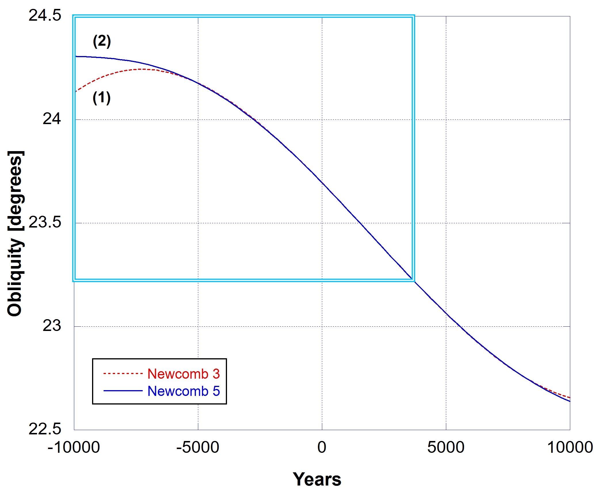
This formula (2) I have used in my analysis. Over the relevant time span from -10,000 years to 2,000 years this formula has sufficient precision for my modelling purposes. See Fig. 2.
These expressions for the obliquity are intended for high precision over a relatively short time span, perhaps several centuries. J. Laskar computed an expression to order T10 good to 0.04″/1000 years over 10,000 years.1
But how could the Newcomb formula be verified? That is, how could you know that it was an accurate representation of the past 10,000 year history of the positions of the planets and other celestial bodies, which effect the Earth’s obliquity?
You can’t know. It is not operational science but historical or forensic science.
Once you get to a point in time (past or future) when you have no actual observational data the model is no longer testable, with one exception. That exception are the small future time increments. That is the purpose of the Astronomical Almanac, to make such predictions on the location of the celestial objects as a function of future time.
However it is impossible to make such predictions over longer times of order 10,000 to 20,000 years into the past and future. Yet this is what is precisely assumed, especially back into the past.
The Earth and solar system were created less than 10,000 years ago, as biblical creationists contend. Then projecting Newcomb’s formula back 20,000 years becomes meaningless.
This all comes down to uniformitarian beliefs about past processes. That is, that the slowly changing positions of the celestial bodies in the solar system can be used to reliably predict past and future positions of celestial objects and hence the obliquity of ecliptic.
Geologists relate past geologic changes, including Earth temperature, over times scales of hundreds of thousands of years, with positions of the planets and the obliquity of the ecliptic as an important contributor to past climate. I will discuss this more later.
Dodwell’s Obliquity Data
In 1980 I was first introduced to the work of former South Australian astronomer George Dodwell, who, over many years prior to 1963, collected historical data on the obliquity of the ecliptic.4 Dodwell developed an hypothesis that some major Earth impact resulted in “a sudden large disturbance of its axis in 2345 BC, and that it reached its present state of completed equilibrium in 1850 AD”.
The year of Dodwell’s impact is very close to the date of the Flood from Ussher’s chronology. According to Bishop James Ussher’s chronology, the Flood occurred in 2348 BC. Ussher calculated that the Earth was created in 4004 BC, and using this as a reference, he determined the Flood happened 1656 years later, which corresponds to 2348 BC. Ussher used the Masoretic Hebrew text for the genealogies of the patriarchs to arrive at the number of 1656 years after creation. This I also have done but I acknowledge that the Septuagint adds about 1500 years to the year of the creation. So I would not be too dogmatic.
In the following I only use Dodwell’s historical obliquity data. You can read his manuscript and decide for yourself about his hypothesis. You might also read a critique by Faulkner published in 2013.5
I have not adopted any of Dodwell’s hypothesis, but only use the “measured” obliquity data, knowing that it probably has errors unknown to Dodwell. One ancient Chinese datum (1100 BC), which is a clear outlier, I have removed.
A Toy Model

The obliquity data I have investigated here with the intention to develop my own model of the creation of the Earth and solar system, with its effect on the global deluge in Noah’s day.
I found it interesting to develop an empirical toy model based on the notion that the initial created state of the planet was an unstable equilibrium with an icy disk of water in equatorial terrestrial orbit. The spheroidal Earth is comprised of a rotating core inside the rotating body of the planet which are not decoupled from each other. I suspect that the icy disk may only have relevance to the period of the Flood. Perhaps not, but modelling needs to be done.
The change in obliquity of the ecliptic may have resulted from the initial creation state of the planet and its core. The planet’s rotation axis is not aligned with the rotation axis of the core as evidenced by the misalignment of the magnetic dipole field axis. The assumption is that the magnetic field is generated from the current in the rotating liquid outer core.
The Earth’s magnetic dipole field axis is tilted by a changing amount around 10° offset from the Earth’s rotation axis, which defines the geographic poles. This means the magnetic field is not aligned perfectly with the Earth’s spin axis. The tilt causes the magnetic poles to be offset from the geographic poles, with the magnetic dipole axis intersecting the Earth’s surface at two points known as the geomagnetic poles.

According to the World Magnetic Model (WMM) and the International Geomagnetic Reference Field (IGRF), the axis of the magnetic dipole is currently inclined at 9.21° to Earth’s rotation axis as of 2025.6
My model includes an initial condition, from the creation process, that introduced a slow change in the polar axis due to a resonant coupling between the planet and the outer core of the planet. There is a coupling between these rotating masses, via angular momentum, which possibly could provide a potential mechanism for the observed change in obliquity.
For this toy model, which I have derived empirically, the obliquity (ε) is the sum of the Newcomb formula (from eq. (2)) plus an additional term Δε:

…. (3)
where T is Julian centuries from the year J2000.0 and t is Julian years, where the time axis has the year zero as 2000 BP.
The anomalous change in obliquity Δε is defined as follows:

…. (4)
where the parameters A, B, Γ and tR are constants to be determined from the fit to the data. The parameters Γ and tR are, respectively, the full-width half maximum and the center of resonance of the Lorentzian. This I’ll call Model 1.
The form of the chosen mathematical model should capture the underlying physics. If the functional form is incorrect the fit will be very poor. It is also important to have as few free parameters (degrees of freedom in the fit) as possible.
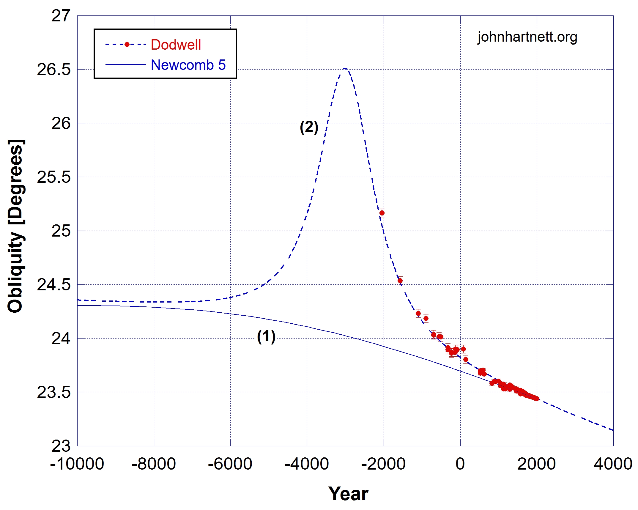
Equation (4) describes a Lorentzian curve that is used in electromagnetic and mechanical resonance phenomena. Here I have used it as a function of time with resonance or reaction time tR. This is summed with the Newcomb(T) term according to eq. (3) and fitted to the Dodwell data for the obliquity of the ecliptic (ε). See Fig. 5.
The measured obliquity (ε) data fit to the model eq. (3) is extremely good with the following parameters determined from the fit.
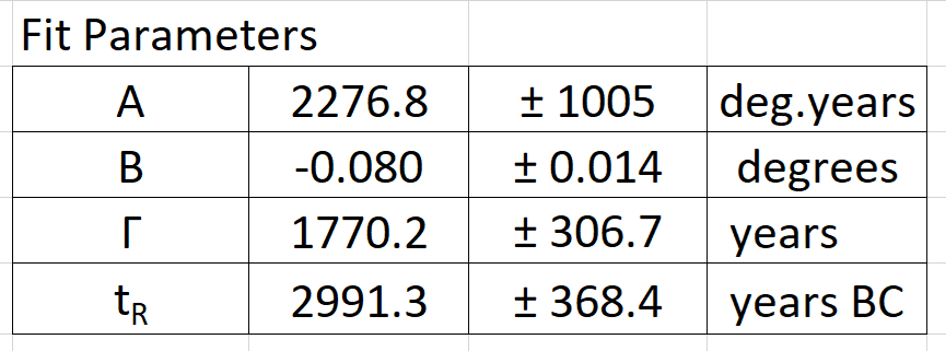
The Model 1 Lorentzian line width (Γ) and the reaction time (tR) are both shown in years BC, meaning before the year zero, hence as negative numbers in Figs 5, 6, 8, 9 and 11. The height of the Lorentzian at time tR is 2A/Γ = 2.57 degrees above the Newcomb background curve (1). That amount represents the maximum departure of the obliquity from equilibrium.
The fit parameters A, Γ and tR have relatively large errors due to the Lorentzian only being constrained on one side of the curve by the available data. But it is worth noting that the curve fit to the measurement data is robust. I also tried a Gaussian, which has an exponential dependence, and no fit could be found. The Lorentzian fit has an R = 0.996 (where R = 1 is a perfect fit) and Chi squared (χ2) = 0.0187 per degree of freedom (where χ2 = 0 is a perfect fit).
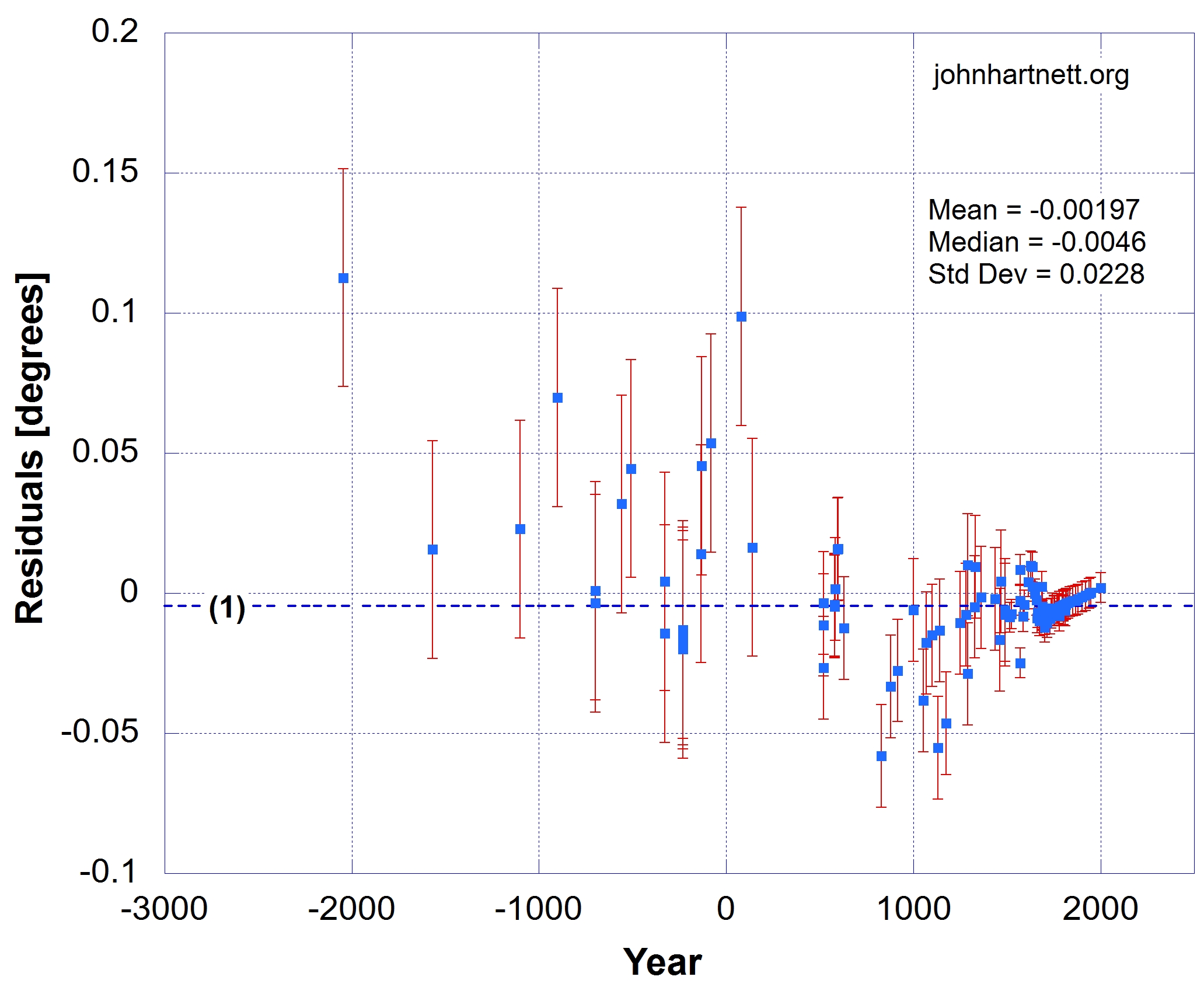
By subtracting the modelled eq. (3) from the Dodwell data we get the residuals as shown in Fig. 5. The error bars shown there are statistical and not error estimates from the measured data. The median of the residuals is -0.0046 and the mean is -0.00197. Except for the three highest value residuals the rest are nearly equally distributed around zero. One problem is the systematics seen in the last 300 years.
The polar axis of the planet not only precesses (P) in a direction counter to the rotation axis (R) at the angle of the obliquity to the ecliptic (ε) but also there is a small nutation (N) in the polar axis. That describes a small ellipse around the mean value of the obliquity (ε). See Fig. 7.
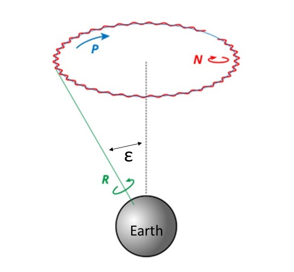
Astronomers have calculated that the precessional cycle of the polar axis completes a full turn over the 26,000 year cycle of the change in the obliquity as shown by Newcomb’s formula in Fig. 2. This is largely due to the Moon and to a lesser extent the Sun. The astronomically measured precession of the equinoxes (P) is about 50 arcsec per year. And the current radius of nutation (N) is 9.63 arcsec = 0.002675 degrees as of April 10, 2025 (Gregorian).7
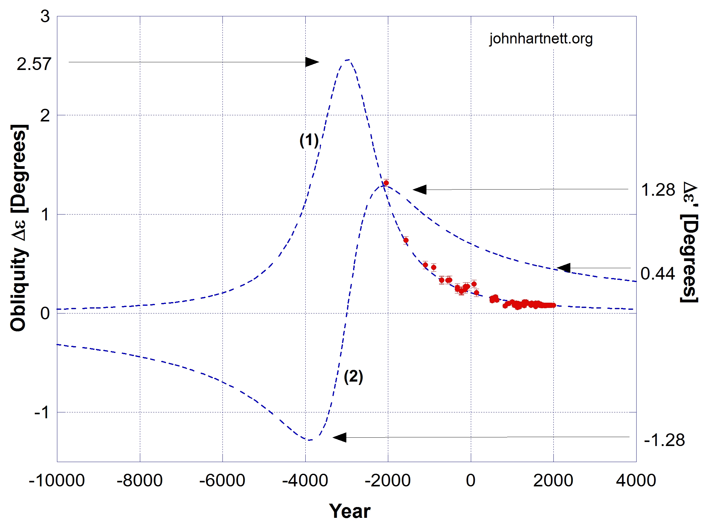
In Fig. 8 I show the change in obliquity Δε away from the equilibrium value of Newcomb’s term in eq. (3). This is described by eq. (4) with all the same parameter values except B = -0.00184.
Also we can write another Lorentzian term, which I designate Model 2, for the change in obliquity, the Δε’ term shown in eq. (5).

…. (5)
where C is an unknown constant. In Fig. 8 this eq. (5) Model 2 Δε’ term with C = A is plotted along with the Model 1 obliquity Δε term.
The currently measured value of nutation is 0.002675 degrees. So in this analysis nutation can be ignored. The maximum values of the Model 2 Δε’ term near years -2000 and -4000 is only about double the present value.
In the following I explore the idea that the Model 2 eq. (5) term Δε’ is related to the spin axis of the liquid iron-nickel core of the planet which is coupled to the rest of the rotating planet though angular momentum.
Geomagnetic Dipole as a Proxy
If we use the current geomagnetic dipole axis as a proxy for the outer core spin axis and its current offset or inclination from the planet’s polar axis of rotation of 9.21° is equivalent to 0.44° deviation in Fig. 8. By adding the difference 8.77° to curve (2) we can calculate the change in the position of the core spin axis with respect to geographical polar axis. This is shown in Fig. 9.
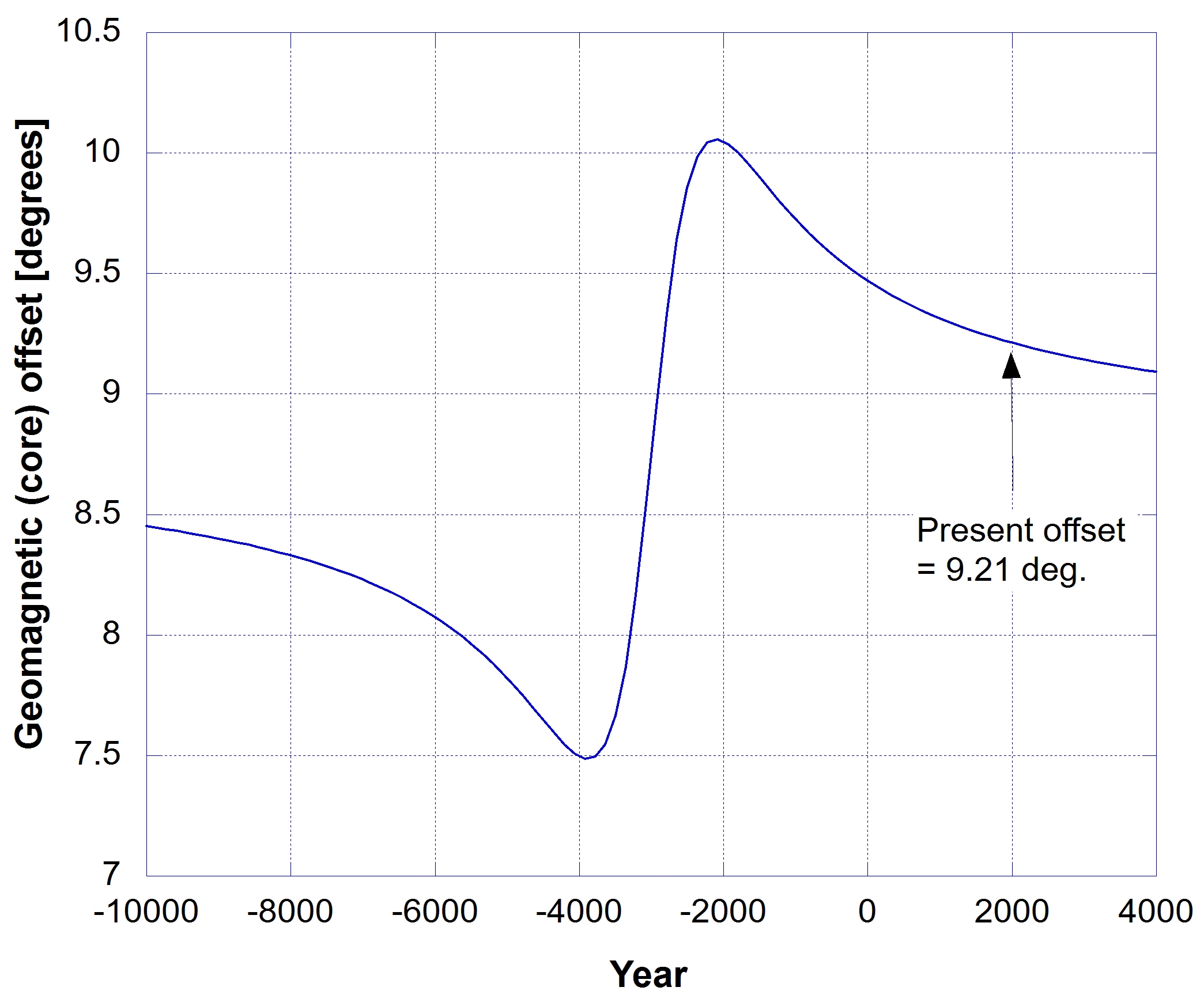
This indicates a decreasing inclination of the core spin axis to the planetary rotation axis, if the offset angle in Fig. 9 is indeed related to the geomagnetic dipole moment. If a correlation with the axial magnetic dipole moment exists we can use it as a proxy for the inclination of the core spin axis.
An analysis of archaeointensity results8 has shown that the Earth’s dipole moment has been higher than the present-day value whilst between 5,000 and 6,000 years ago it was much weaker.9
We should expect to see a dependence in the measured values for the Virtual Axial Dipole Moment (VADM). Here VDM indicates the data are averaged as shown in Fig. 10.
I have used the global average VADMs from Table II of (Yang et al, 2000),9 which combined old and new published data from their Table I. I have plotted the average VADM data against the core spin axis dependence shown in Fig. 9 assuming a correlation with the dipole moment. The result is shown in Fig. 10. The scaling factor C = 1.256A and an added offset 9.118 is required for the fit. Of course the units are different but the assumption of a linear relationship between VDM and Δε’ from eq. (5) seems to work.
Table II of (Yang et al, 2000) indicates the number of samples and the time intervals over which they are averaged. In Fig. 10 the error bars on the time axis is the date range of the samples averaged together and the VDM error bars are the statistical 1σ spread of the data around their mean values.

The residual of the fit R = 0.744 indicates a good fit. Visually even though the data are noisy there is overlap of the 1σ errors for nearly all data. This indicates a general agreement with the hypothesis.
The fit for data in years less than -3,000 is very good. However, if the line width Γ is allowed to be a free parameter in Fig.10 the fit over all the data is improved significantly with R= 0.858 and the line width Γ becomes 2.69x the value of 1770.2 years determined from the fit in Fig. 3.
If there is a direct connection between the inclination of the core spin axis and the planet’s obliquity to the ecliptic via a resonance process the line width should be the same. A mechanism needs to be found that can explain the relationship in Fig. 8. That will require some investigation. Nevertheless, it looks very promising.
Global Temperature Changes
Another interesting feature of this toy model is when the total obliquity ε, which includes the Newcomb formula and the Model 1 Δε term (eq. 3), is compared with typical Greenland ice-core-proxy-derived temperatures a correlation appears. See Fig. 11.

In Fig. 11 though there is an apparent correlation between Newcomb’s formula (1) and the ice-core temperatures (3) there is a better correlation with Dodwell obliquity data and curve fit (2). The relationship to Newcomb’s formula is often cited by geologists trying to explain Greenland ice-core derived temperatures over much longer geologic timescales than shown here.
One comment worth making here is that though we don’t have a measure of the quality of Dodwell’s Table of obliquity data the fit to Model 1 described by eqs (3) and (4) would have to be considered truly remarkable if the data had no real underlying physical trend.
Concluding remarks: There seems to be sufficient information from this brief analysis of Dodwell’s data and how it fits a Lorentzian line shape, to merit further investigation. The curve fit seems to indicate some type of long timescale mechanical reaction or resonance around the year 2991 ± 368 BC. That means some gravitational or mechanical mechanism caused an anomalous deviation of the obliquity of the Earth’s rotational axis away from equilibrium and then its recovery. I propose that it was related to the initial creation state of the Earth and the angular momentum differences in the core, the planet and the “waters above”. The mechanism may be connected to Earth changes during the great deluge in the time of Noah. See Related Reading listed below.
Also read my follow up piece Can We Know the Year of Noah’s Flood?
This is a work in progress. Stay turned for more developments.
References
- https://en.wikipedia.org/wiki/Ecliptic
- https://en.wikipedia.org/wiki/Ephemeris
- U.S. Naval Observatory, Nautical Almanac Office; H.M. Nautical Almanac Office (1989). The Astronomical Almanac for the Year 1990. U.S. Govt. Printing Office. ISBN 0-11-886934-5., p. B18
- George F. Dodwell B.A., FRAS, The Obliquity of the Ecliptic, Ancient, mediaeval, and modern observations of the obliquity of the Ecliptic, measuring the inclination of the earth’s axis, in ancient times and up to the present. Manuscript here: https://www.barrysetterfield.org/Dodwell/Dodwell_Manuscript_1.html Data Table here: https://www.barrysetterfield.org/Dodwell/Dodwell_data.html
- D.R. Faulkner, An Analysis of the Dodwell Hypothesis, Answers Research Journal 6 (2013): 179–191, https://answersresearchjournal.org/analysis-of-the-dodwell-hypothesis/
- https://www.ncei.noaa.gov/products/wandering-geomagnetic-poles
- https://www.neoprogrammics.com/obliquity-of-the-ecliptic/
- McElhinny M.W. Senanayake W.E.,1982. Variations in the geomagnetic dipole 1, the past 50 000 years, J. Geomag. Geoelectr., Vol. 34, Issue 1, pp. 39– 51, https://doi.org/10.5636/jgg.34.39
- S. Yang, H. Odah, J. Shaw, Variations in the geomagnetic dipole moment over the last 12 000 years, Geophys J Int, Vol. 140, Issue 1, January 2000, pp. 158–162, https://doi.org/10.1046/j.1365-246x.2000.00011.x https://academic.oup.com/gji/article/140/1/158/707986
Related Reading
- The Physics of Creation | Day 1
- The Physics of Creation | Day 2
- The Physics of Creation | Day 3
- The Physics of Creation | Day 4
- The Physics of the Global Flood
Free Subscribers
Subscribe to our Newsletters as a Free Subscriber and be notified by email. Just put your email address in the box at the bottom of your screen.
You’ll get an email each time we publish a new article. It is quick and easy to do and totally free. You only need do it once.
Premium Subscribers
Subscribe to our Newsletters as a Premium Subscribers at $5 USD/month or $30 USD/year (you choose).
Paid Premium Subscribers will get exclusive access to certain content I publish, which I expect to be about 4 exclusive posts per month. That will only cost you a cup of coffee per month.
Also you’ll get access to download, for free, a PDF of my book Apocalypse Now. You can download it from a Premium members only post here.
And now you’ll get exclusive access to the chapters (in their initial draft form) to my new book with working title “The Physics of Creation”; plus eventually a PDF of the final compiled book.
This is how you can support my work. I have been publishing this website for 10 years now and up to 2024 I never asked for any support.
Press the button “Premium” on the front page to find a list of Premium content. Over time that list will grow. Thanks so much to all supporters.
At a minimum, please join as a Free Subscriber. It’ll cost you nothing. It may also help me beat the shadow banning of some posts.


Leave a comment