

At some time in the past 8,000 years the planet Earth rocked and reeled on its polar rotational axis. The question is, did that coincide with Noah’s flood? And if so, can we determine from observational data when that was?
For an introduction read Obliquity of Earth’s Axis | How Has It Changed?
When further thinking about the historical obliquity of the ecliptic data, that is, tilt of the Earth’s axis, as collated by South Australian astronomer George Dodwell,1 which seems to have some validity to the past Earth changes around the time of the great deluge, the following passage from the book of Isaiah came to mind.
18 And it shall be, he who flees from the sound of terror shall fall into the pit. And he who comes up out of the midst of the pit shall be taken in the snare. For the windows from on high are opened, and the earth’s foundations quake. 19 The earth is breaking, breaking! The earth is crashing, crashing! The earth is tottering, tottering. 20 Like a drunken one, the earth is staggering, staggering! And it rocks to and fro like a hut. And its transgression is heavy on it; and it shall fall, and not rise again.
Isaiah 24:18-20 KJ3
It is possible that this passage of scripture uses the same language as used of the great Flood. The transgressions or sins of man were great before the Flood as they were at the time of the prophet Isaiah. The windows on high (of heaven) are opened and the Earth’s foundations quake (were broken up).
The Earth here is a reference to the inhabitants but this may be an application of what physically happened at the Flood. The prophet would have been well familiar with the Flood events and he used the same language.
If so, the tilt of the Earth’s rotational axis may have changed. An increase means a greater angle from the normal to the ecliptic and a decrease means a lesser angle. This would make the differences in the seasons, summer and winter, more or less significant depending on the extent of that change (Psalms 74:17).
This led me to have a further look at the model I was using to describe the historical obliquity changes over the last 8,000 years. If the planet reeled or rocked “to and fro like a hut” then obliquity may have changed in both directions. As a result I now propose a third model (Model 3) in my description of this period of time.
Previously2 I used the 5th order polynomial to model gradual change in the obliquity (ε) of the Earth’s rotational axis as it precesses over its 26,000 year cycle due to the gravitational pull of the Moon, Sun and the planets of the solar system, with importance in that order. That equation, named after Simon Newcomb is specified by the Astronomical Almanac for 2010 as:
Newcomb(T) = 23°26′21.406″ − 46.836769″ T − 0.0001831″ T2 + 0.00200340″ T3 − 0.576×10⁻⁶″ T4 − 4.34×10⁻⁸″ T5, … (1)
where T is Julian centuries from the year J2000.0.
My empirical models are of the form
ε= Newcomb(T) + Δε(t), … (2)
where the obliquity of the ecliptic (ε) is the sum of the Newcomb formula (from eq. (1)) and an additional anomalous term Δε. Here T is Julian centuries from the year J2000.0 and t is Julian years, where the time axis has the year zero at 2000 BP (Before Present).
Model 1: The anomalous change in obliquity Δε was defined as follows:

… (3)
Now I propose a new model, labelled Model 3 because my previous paper had a Model 2 also.
Model 3 is also Lorentzian and is essentially the time derivative of the Model 1 formulation.
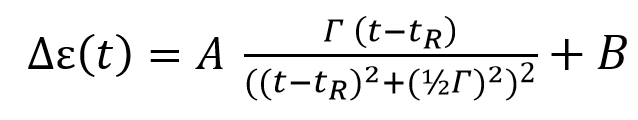
… (4)
where the parameters A, B, Γ and tR are constants to be determined from the fit to the data. The parameters Γ and tR are, respectively, the full-width half maximum and the center of resonance of the Lorentzian line.
Equation (4) describes a Lorentzian curve that is used in electromagnetic and mechanical resonance phenomena. Here I have used it as a function of time with resonance or reaction time tR. This is summed with the Newcomb(T) term according to eq. (2) and fitted to the Dodwell data for the obliquity of the ecliptic (ε). See Fig. 2.

The measured obliquity (ε) data fit to the model eq. (2) with Model 3 from eq. (4), is extremely good with the following parameters determined from the fit. This Model 3 fit gives an improved quality of fit compared to the Model 1 Lorentzian line.

The Lorentzian line width (Γ) and the time of resonance (tR) are both shown in years BC, meaning before the year zero, hence as negative numbers. The Lorentzian line varies from a minimum of -1.56° to +1.64° from the crossing point of the Newcomb background curve (1) at time (tR). The total of 3.2° represents the range of departure of the obliquity from equilibrium.
This behaviour seems to be somewhat more of a description of Isaiah 24 passage, compared to the Model 1 description but that is subjective. I make no scientific argument from Isaiah 24.
In terms of the quality of the fit here I plot the residuals after the modelled curve (2) in Fig. 2 has been subtracted off the Dodwell data. See Fig. 3.

The residuals are better distributed about zero with a median value -0.00064, much closer to zero than the Model 1 result.
This Model 3 gives a greatly improved value for the reaction or resonance time (tR), and if this is the year of Noah’s flood, it occurred in year 3154 ± 191 BC. The Model 1 fit to the same data yielded a much wider range in the errors of 2991 ± 368 BC. Though these dates are still consistent with each other, the Model 3 result more strongly excludes Bishop Ussher’s date for the Flood in 2348 BC.
Ussher used the Hebrew Masoretic Text (MT) for the genealogies of the patriarchs from Genesis 5 and 11 to arrive at the number of 1656 years after creation for the Flood. But I acknowledge that the Greek Septuagint (LXX) adds about 1500 years to the year of the creation. From that Henry B. Smith, Jr puts the Flood year at 3298 BC using the LXX.3
The time where the Model 3 curve crosses the Newcomb background curve in the year 3125.8 BC and the maximum rate of change of the obliquity is 15.73 arcsec per year in the year 3136.2 BC, which is a little later than the reaction time (tR) because of the changing tilt due to Newcomb’s formula.
Using the reaction time (tR) as the year of the Flood I calculate that the change in the obliquity (ε) that occurred in the preceding 120 years was +0.5 degrees. That means the tilt increased towards the background Newcomb value. A half degree change in tilt must have been a significant warning to those who saw Noah building the Ark (Genesis 6:3). The rate of change was also increasing. It would have been a pending warning for what was coming.
The result here is significantly different to what biblical creationists have proposed in the past, suggesting most of the change in the polar axis occurred in the Flood year. In this model the change is much slower and started at the end of creation week. I do not yet know what cause this anomaly to occur but it was built-in to the creation, an unstable equilibrium condition, that the Creator used as He has foreknowledge of all future events (Isaiah 46:10).
In an effort to find a mechanism want to model a disk of “waters above” in terrestrial orbit from the creation to see if that could produce the changes seen in Fig. 2. But before I started to model that, I first looked at the core of the planet.
Effect on Core Rotation Axis
In the following I extend my toy model to include the effect on the rotation axis of the core of the planet. Since the outer core is a liquid (by design) I assume that it freely rotates with respect to the mantle above it. See Fig. 4.
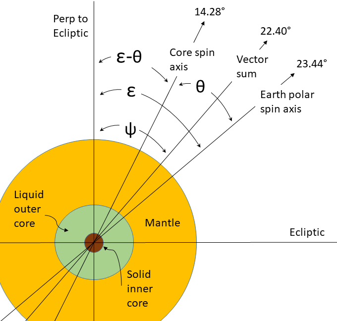
From here on I assume that the geomagnetic poles are defined by the magnetic dipole field generated by a current in the liquid Iron-Nickel outer core in free decay due a finite electrical resistance. Therefore the spin axis of the core is connected to this dipole field. The current inclination of the geomagnetic poles is θ = 9.21° from the Earth’s rotational axis.
The Earth’s polar spin axis is currently at ε = 23.44° from the Ecliptic, therefore the core spin axis is at an angle (ε-θ) = 14.28° from the Ecliptic.
For the modelling here we have two conservation equations:
- Conservation of energy

… (5)
where IE is the moment of inertia for the Earth, IM the moment of inertia for the mantle and crust, and Ic is the moment of inertia for the core, where both inner and outer core have been spinning together since the end of creation week nearly 8000 years ago.
The parameters ωE, ωM and ωc are respectively the angular rotation speeds of the Earth, mantle and core. The rotation speed which we measure I am calling the rotation speed of mantle equal to the rotation speed of the Earth ωM = ωE = 2π/(1 day) where 1 day = 23 hours and 56 minutes. That is the rotation period with respect to the stars. You get an extra 4 minutes when measured with respect to the Sun.
I assume that since creation, that is, over the timescale of 10,000 years very little energy has been lost from the total rotational energy (IEωE2 ) of the system. Therefore we can assume in the following that ωE = ωc = ωM and also that these are constants.
2. Conservation of angular momentum

… (6)
where barred symbols denoted with e_subscript are vectors.
Dividing (6) by constant the angular frequency where ωE = ωc = ωM eq. (6) becomes

… (7)
The vector eM points in the direction of the observed obliquity angle ε, whereas the vector ec points in the core spin axis direction at an angle of (ε-θ) from the Ecliptic. The current value is 14.28°. The sum of these two vectors, eE, point in the direction at an angle of ψ from the Ecliptic. See Fig. 4. The angle ψ and its tangent are constants due to conservation of angular momentum. Summing the vectors we get:
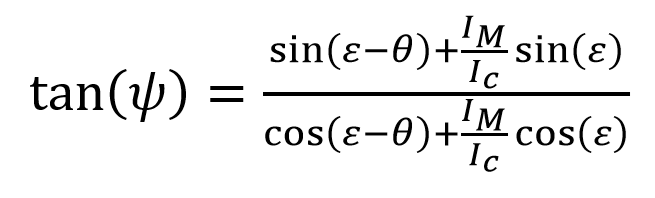
… (8)
where the angle ψ is constant.
Expanding eq. (8) with a trigonometric identity

… (9)
This eq. (9) is quadratic in sin(θ) and can be solved analytically. I have used the software Mathematica® to do this and derived the changing value of the angle θ. But the expression is too complex to write here.
The following is simpler, where I have made a simplifying assumption for small θ, cos(θ) ≈ 1, then solved for sin(θ).

… (10)
This gives us a function of the core inclination (θ) as a function of obliquity (ε); it is very close to the full analytic solution. Since tan(ψ) is constant we can calculate its value at the present time from eq. (8).
The moments of inertia are for the spherical bodies:
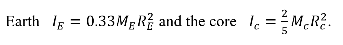
Assuming perfect decoupling between the mantle and crust at the liquid outer core interface I assume the mantle rotates separately from the core in the first approximation. Thus the ratio

… (11)
because the core mass Mc is 32.6% of total Earth mass ME and the Earth radius RE = 1.84Rc.
From eqs (8) and (11) tan(ψ )=0.412 radians and ψ = 22.40°. As expected only about 1° less than the polar rotation axis angle. In practice, I used the full analytic solution and had to adjust IM/Ic = 7.9 to get the angle θ = 9.21° at the present time, which is the measured value.
Now, by using eq. (10) and the known constants we get the value of the core inclination to the geographic polar axis. See Fig. 5.

As expected to compensate for the vector change in the angular momentum the smaller mass of the core needs to change by a greater degree to the change in the geographical polar rotation axis.
Now one more comparison can be made.
Assuming as I have that the geomagnetic dipole field in generated by the rotation of the core, the dipole magnetic moment should be related to the changes in the core axis inclination.
The magnetic dipole moment is a measure of the strength and orientation of a magnet or other object that exerts a magnetic field. It determines the torque experienced by the object in a given magnetic field, and the strength of this torque depends on both the magnitude of the magnetic moment and its orientation relative to the magnetic field.
In the following I have used measured data of the Virtual Axial Dipole Moment (VADM) determined by archeointensity measurements. I have used the global average VADMs from Table II of (Yang et al, 2000),4 which combined old and new published data from their Table I.
On double-Y plots in Figs 6a and 6b I show the core inclination angle compared to the averaged VADM measurements. Fig. 6a is for Europe only data and Fig. 6b is for all world-wide data.
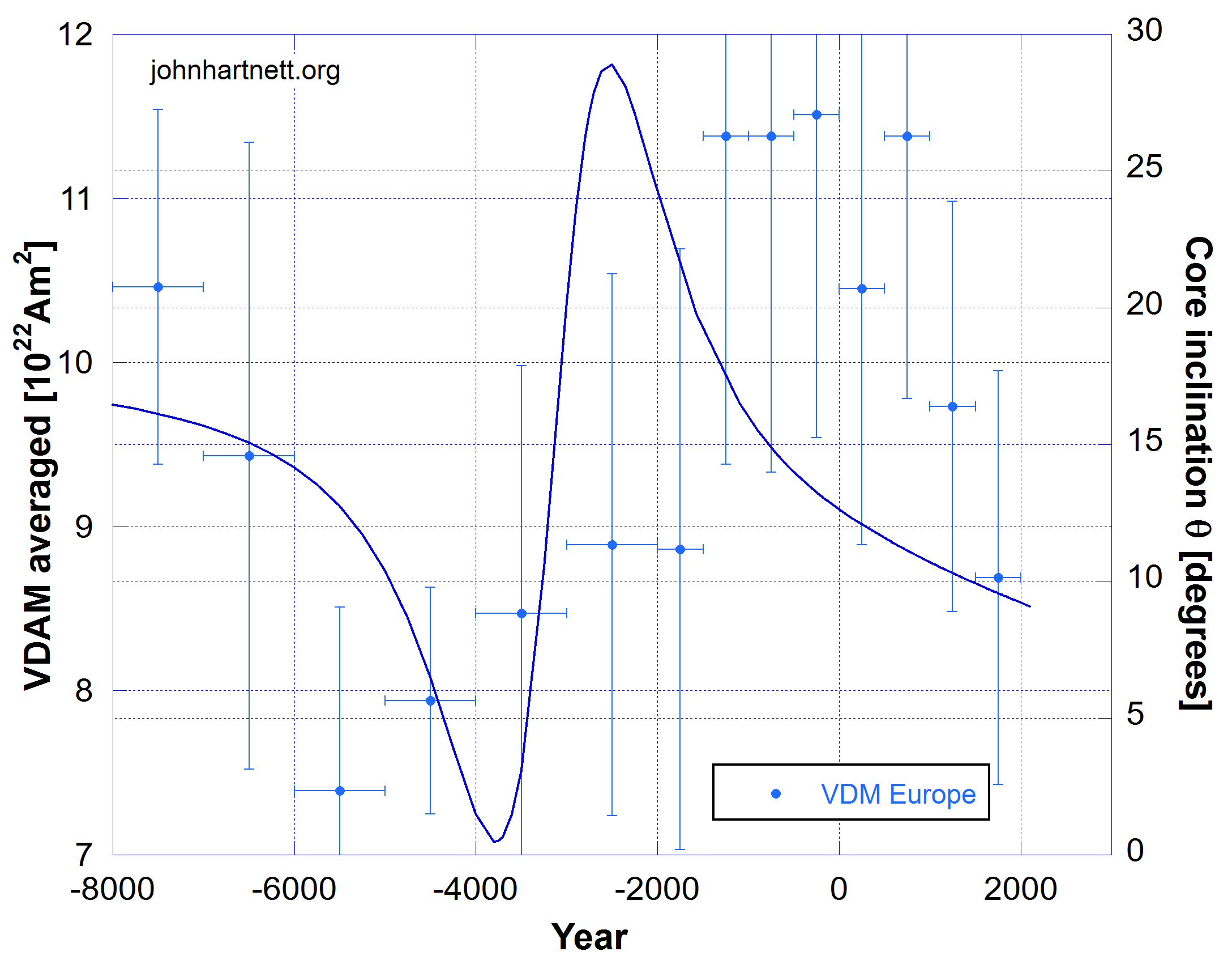

The correlation is far from perfect but it has the correct functional form.
What needs to be done now is modelling on how the changing core inclination correlates to changes in the axial dipole magnetic field. I suspect the effects would have been very significant because the change in core inclination is much greater than the change in the planet’s obliquity.
During the periods of greatest inclination changes the currents in the outer core would have been disturbed and turbulence would have been very significant.
I suggest also that from the end of creation week, the magnitude of the core current (in Amps) was in exponential decay, due to the finite electrical resistance of the liquid Iron-Nickel metal, resulting in the intensity of the magnetic field decaying. But the rotation of the core has essentially not changed. The former is due to electrical resistance in the outer core but the latter is mechanical in nature; really it is fluid dynamic in nature.
Of course my assumption of no mechanical coupling losses between the outer core and the mantle needs also to be modelled. A small mechanical resistance there would slow the core angular speed and angular momentum and rotational energy would no longer be conserved.
Any losses I expect would show up as an increase in core entropy and thus heat. Certainly that is occurring with energy being lost from the intensity of the magnetic field, which has been measured to be decaying exponentially for the past 200 years.
Conclusion
There is a quite incredible issue here! If Dodwell’s historical obliquity data, all collected before 1963, is of no credibility as some creationist and secular scientists have suggested, then how do you explain the quality of the curve fit in Fig. 2? To state that it was by chance is beyond credibility.
And Dodwell’s could not have fudged that data. For one thing he made no reference to any type of Lorentzian curve fit, but used a Log sine curve for his analysis. His model was very different because as I believe he was led by an effort to get the year of the Flood to align to Bishop Ussher’s chronology.
In my analysis I have allowed the functional form of the fitted curve, which describes the underlying physics, to determine the year of the Flood. That resulted in 3154 ± 191 BC. This was from my second model applied to the Dodwell data (called Model 3 for other reasons). This result is consistent with my Model 1 determination of 2991 ± 368 BC but inconsistent with Bishop Ussher’s date for the Flood in 2348 BC. In fact, it is excluded.
In the latter part of this research I developed a toy model to test the interplay of the spin axes of the planet (really the mantle) and the core. That has led to the idea that the core spin axis changed by a factor of 9 compared to the 3.2 degree change in the planet’s rotation axis. Such large changes even over the timescale of thousands of years must have had a significant effect of the Earth geomagnetic field. That is the subject of my ongoing research. But the reasonably good correlation between changes in the core spin axis and the Earth’s axial dipole moment from archeointensity measurements also needs an explanation.
Finally a mechanism needs to be found that caused the anomalous change in obliquity of the polar rotation axis over the past 8,000 years.
References
- George F. Dodwell B.A., FRAS, The Obliquity of the Ecliptic, Ancient, mediaeval, and modern observations of the obliquity of the Ecliptic, measuring the inclination of the earth’s axis, in ancient times and up to the present“. Manuscript here: https://web.archive.org/web/20180414005516/http://www.setterfield.org/Dodwell/Dodwell_Manuscript_1.html Data Table here: https://web.archive.org/web/20180415103250/http://www.setterfield.org/Dodwell/Dodwell_data.html
- J.G. Hartnett, Obliquity of Earth’s Axis | How Has It Changed?, https://biblescienceforum.com/2025/04/17/obliquity-of-earths-axis-how-has-it-changed/
- Henry B. Smith Jr, The Case for the Septuagint’s Chronology in Genesis 5 and 11, https://digitalcommons.cedarville.edu/icc_proceedings/vol8/iss1/48/
- S. Yang, H. Odah, J. Shaw, Variations in the geomagnetic dipole moment over the last 12 000 years, Geophys J Int, Vol. 140, Issue 1, January 2000, pp. 158–162, https://doi.org/10.1046/j.1365-246x.2000.00011.x https://academic.oup.com/gji/article/140/1/158/707986
Related Reading
- Obliquity of Earth’s Axis | How Has It Changed?
- The Physics of Creation | Day 1
- The Physics of Creation | Day 2
- The Physics of Creation | Day 3
- The Physics of Creation | Day 4
- The Physics of the Global Flood
Free Subscribers
Subscribe to our Newsletters as a Free Subscriber and be notified by email. Just put your email address in the box at the bottom of your screen.
You’ll get an email each time we publish a new article. It is quick and easy to do and totally free. You only need do it once.
Premium Subscribers
Subscribe to our Newsletters as a Premium Subscribers at $5 USD/month or $30 USD/year (you choose).
Paid Premium Subscribers will get exclusive access to certain content I publish. That will only cost you a cup of coffee per month.
Also you’ll get access to download, for free, a PDF of my book Apocalypse Now. You can download it from a Premium members only post here.
And now you’ll get exclusive access to the chapters (in their initial draft form) to my new book with working title “The Physics of Creation”; plus a PDF of the final compiled book.
This is how you can support my work. I have been publishing this website for 10 years now and up to 2024 I never asked for any support.
Press the button “Premium” on the front page to find a list of Premium content. Over time that list will grow. Thanks so much to all supporters.
At a minimum, please join as a Free Subscriber. It’ll cost you nothing. It may also help me beat the shadow banning of some posts.


Leave a comment