Bible Science Forum

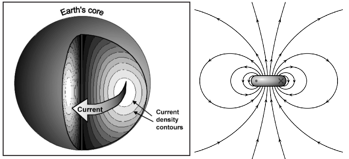
The Young Earth Creation model of the Earth’s magnetic field was developed by Dr. Thomas Barnes¹ and then built on by Dr. D. Russell Humphreys. The model posits that the geomagnetic dipole field is generated by a current in the liquid Iron-Nickel outer core of the planet. Due to the finite electrical resistance of the core the magnetic field strength (denoted B and measured in units of gauss or Tesla) has been decreasing over the past 200 years since Carl Friedrich Gauss made the first measurements. See Humphreys “The Earth’s Magnetic Field is Still Losing Energy”² for an excellent introduction to the subject.

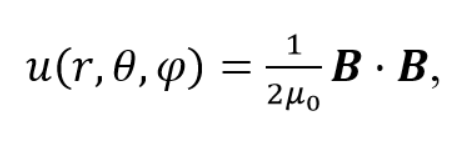
The model on the right in Fig. 1b is a standard dipole field generated from a circulating current loop in the ring in and out of the page. This is essentially the Barnes-Humphreys model as shown on the left in Fig. 1a.

The Barnes-Humphreys model very successfully explained the decay in the magnetic field strength due to the resistance losses in the core resulting in ohmic dissipation also called ‘joule heating’. The historical measurements of the magnetic B–field, the dipole field represented by Fig. 1b,for Earth, indicate it is young. Read on.

The long age evolutionists acknowledge that the dipole field is decaying as a function of time but they argue for a putative dynamo that over billions of years regenerates the decaying B–field. They argue that the energy lost from the dipole field is being stored in the non-dipole field modes, such that the total energy is roughly constant. Then at a later date that energy comes out of the non-dipole B–field and goes back into the dipole B–field, regenerating it. But that is wishful thinking.

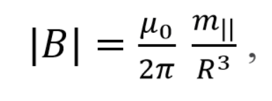
The energy density (u) (in units J/m³) stored in the magnetic B–field at a given point is

where r, θ, φ are radial and angular spherical coordinates. The dot represents the scalar product, and μ₀ is the magnetic permeability of the vacuum (which is essentially the same as the magnetic permeability of the Earth).

Humphreys integrated the measured B-field components over the volume of the Earth and calculated the total energy in both the magnetic dipole field and the non-dipole field modes. His results are shown in Fig. 2a for the period 1900 to 2000 and Fig. 2b for the period 1960 to 2000. The total energy is the sum of the dipole and non-dipole energies.

Using non-linear regression curve fitting with this equation for the energy,

we get the following parameters for best fits. The exponential with base 2 was chosen so that the half-life (time for halving of the energy) is easily seen. The best fit parameters (A, t₀) for curve fits from Fig. 2 are listed in Table I.

Table I Best fit parameters

The quality of fit is expressed by the residual R, which for a perfect fit R=1. The data for the period 1960 to 2000 show better curve fits as indicated by the R parameters. Humphreys wrote that after 1970 the errors were also better than for data before that period. I have used data after 1960 because the systematics looked pretty good from 1960 onwards.

Even though the non-dipole energy shows an increase, the dipole energy and the total energy (the sum of the dipole and the non-dipole components) show a decrease. From the 1960-2000 data the dipole B-field halves its energy every 439.8 ± 7.3 years and the total energy halves every 1,351.4 ± 128.7 years. This is consistent with the commonly stated figure of a half-life of about 1,400 years. This figure is based on the most reliable data and unless some new data comes to light there is no reason to assume that the energy lost from the magnetic field will not continue.

One YEC argument for the young age of the Earth is that if you project backwards in time 10,000 years the dipole energy would have been 5 x 10⁶ times the present value, or 30 million exajoules (EJ) = 3 x 10²⁵ J. 1 EJ was the energy released by the 2011 Tōhoku earthquake and tsunami. However if you assume the wider data 1960-2000 is more reliable and instead use the time constant of 3,391± 1,729 years, the dipole energy would have been 147 times the present value 10,000 years ago. Either way the energies would have been very unphysical for the Earth.

Having said that, in what follows, I show that the energy in the dipole was not extremely high more than 5,000 years ago. In fact the exponential fits that Humphreys used and I have repeated here are unnecessary as a linear fit will do. A decreasing trend but I now believe from what follows is that it is not valid to assume an exponential trend back in time.

The argument that the energy moves from the dipole B-field into the non-dipole field modes and back again over geological time is not based on any observed facts. The total energy of the magnetic field has been observed to be decaying over the past several hundred years. That is an observational fact. But also it is worth remembering that the dipole B-field energy has been halving every 439.8 ± 7.3 years. That is from a sample time of 40 years, which is very short compared to the time since creation, which must be less than 8,000 years.

Axial Magnetic Moment

The axial magnetic moment refers to the magnetic moment of a magnet measured along its axis, typically from the north pole to the south pole. The magnetic field at a point on the axial line due to a circulating current loop in a direction perpendicular to the plane of the circulating current is described by:

where μ₀​ is the permeability of free space, m_|| is the axial magnetic dipole moment of the magnet; the subscript || indicates the axial magnetic moment. The magnetic moment is measured at a distance x from the center of the magnet, where x >> r, the radius of the circulating current. In our model the radius r is that of the liquid outer core. And in our case x = R is the radius of the Earth; the surface is where all measurements are made.

The magnetic moment has units of [Am²] and the B-field units of Tesla, which in SI units is [kg s^-2 A^-1]. The permeability of the Earth is very close to that of free space μ₀ = 4π x 10^-7 kg m s^-2A^-2.

From eq. (1) we can write the magnitude of the B-field in terms of the energy density u.

For the magnitude of the axial magnetic moment m_|| at the surface of Earth of radius R eq. (3) becomes

To first approximation we replace the energy density u with the energy in the dipole (E_d) divided by the volume of the Earth.

And solving for the magnitude of the axial magnetic moment we get

which may be inverted to get the energy in the dipole in terms of the magnitude of the axial dipole moment.

Using eq. (8) I calculated the equivalent energy in the dipole using the published axial magnetic moments called the Virtual Axial Magnetic Moment (VADM) determined by archeointensity measurements. The global averaged data from Table II of (Yang & Odah, 2000)³ were used. The result is shown in Fig. 3.

To plot the energies converted from VADM magnetic moment data it was necessary to scale the result by a factor of 3. This probably was due to my approximation. As a result the trend in the (black) dipole energy data converted from (Yang & Odah, 2000) align well with the (red) dipole energy data from Humphreys. See my Fig. 2.

Caution is advised here that we do not extrapolate the non-dipole and hence the total energy back in time as some have done to set an upper limit on the energy in the dipole. The total energy does have an upward trend back in time but what we have here is a tiny fraction of the whole range (10,000 years). Since we have no historical data for the non-dipole energies anything else we do with those data will involve speculation.

Also please note: I do not accept the uniformitarian timescale used in the published VADM data. The timescale for older dates should be compressed by 25% or more. So keep that in mind as I use it in the following 2 figures.

However there is a lot we can learn from Fig. 3. The dates of the archeointensity measurements have broad statistical errors as they should, but because of the unknown uniformitarian assumptions we need to consider that there may be some compression needed in the timeline.

Nevertheless we can conclude that dipole and total energy cannot be extrapolated back in time to reach unphysical values as has been used by creationists. Yet Humphreys’ dipole energies match the trend line in the VDM data for about the last 1,000 years. 

The indication is that the energy in the dipole has decreased recently but increased since creation. The minimum energy occurred somewhere near the great Flood. With the Earth changing its axial tilt and the subsequent change in the inclination of the core rotation axis I would expect strong disturbances in the liquid Iron-Nickel outer core. See Refs 4, 5.

Using eq. (7) I converted Humphreys’ dipole energy data into axial magnetic moments and compared the result to the published VADM data of (Yang & Odah, 2000) in Fig. 4. It was necessary to do the same scaling as in Fig. 3, but this time by the square root of the factor 3 used before.

Fig. 4 contains the same data as Fig. 3 but represented in a different form. These two figures offer a consistent interpretation that as the Earth’s core underwent a major change in the direction of its rotation axis (by as much as 30 degrees) major changes occurred in the axial magnetic moment. Those changes started to occur at the beginning of creation and they left their mark on the whole planet.

The year of the great Flood is indicated on Figs 3 and 4, with error bounds from the curve fit that determined it to have occurred in the year 3,154 ± 191 BC. But Earth changes were well under way long before that time.

The axial magnetic moment of the planet is now back to the value it started out with. This is a confirmation that the massive change in the obliquity of the rotation axis and in the core axis has essentially stabilized.

Starting around 7,500 BC (uncorrected for uniformitarian assumptions) the tilt of the Earth’s rotation axis began rising (actually decreasing its angle to the ecliptic) and after reaching about 1.5 degrees less than it started with, it fell, i.e. increased by about 3 degrees and then returned to near its starting obliquity. See Ref 5.

At the same time the tilt in the core axis changed by about 9 times that amount which had a profound effect on the magnetic field of the planet. The geomagnetic poles reduced their magnetic strength initially but after the period around the global Flood their strength increased, peaked and has been reducing since then, that is, over the past 1,000 years. See Figs 3 and 4.

During the period of the major changes to the core spin axis (5,000 BC to 1,000 BC; Fig. 5 of Ref. 5). A lot of energy flowed out of the main axial dipole into the non-dipole modes of the magnetic field. This is indicated by the period before the global Flood in Fig. 3. Turbulence in the non-dipole moments would have meant rapid changes to even the polarization of the magnetic B-field at the surface. Humphreys suggested that this occurred during the Flood but I am suggesting here that it did happen but over many millennia before and after the Flood.

References

1. T.G. Barnes, 1973. Electromagnetics of the earth’s field and evaluation of electric conductivity, current, and joule heating in the earth’s core. CRSQ 9:222–230.
2. D. R. Humphreys, 2002. The Earth’s Magnetic Field is Still Losing Energy, CRSQ 39:3–13; https://www.creationresearch.org/crsq-2002-volume-39-number-1/crsq-2002-volume-39-number-1_earth-s-magnetic-field
3. S. Yang, H. Odah, J. Shaw, Variations in the geomagnetic dipole moment over the last 12 000 years, Geophys J Int, Vol. 140, Issue 1, January 2000, pp. 158–162, https://doi.org/10.1046/j.1365-246x.2000.00011.x  https://academic.oup.com/gji/article/140/1/158/707986
4. Obliquity of Earth’s Axis | How Has It Changed?
5. Can We Know the Year of Noah’s Flood?

---

Related Reading

• Obliquity of Earth’s Axis | How Has It Changed?
• Can We Know the Year of Noah’s Flood?
• The Physics of Creation | Day 1
• The Physics of Creation | Day 2
• The Physics of Creation | Day 3
• The Physics of Creation | Day 4
• The Physics of the Global Flood
• My Book ‘Physics of Creation’

---

Free Subscribers

Subscribe to our Newsletters as a Free Subscriber and be notified by email. Just put your email address in the box at the bottom of your screen.

You’ll get an email each time we publish a new article. It is quick and easy to do and totally free. You only need do it once.

---

Premium Subscribers

Subscribe to our Newsletters as a Premium Subscribers at $5 USD/month or $30 USD/year (you choose).

Paid Premium Subscribers will get exclusive access to certain content I publish. That will only cost you a cup of coffee per month.

This is how you can support my work. I have been publishing this website for 10 years now and up to 2024 I never asked for any support.

Press the button “Premium” on the front page to find a list of Premium content. Thanks so much to all supporters.

---

At a minimum, please join as a Free Subscriber. It’ll cost you nothing. It may also help me beat the shadow banning of some posts.

---

Comments Welcome Below