

Here I present further developments as I explore my toy biblical creation model wherein the Earth’s axis suffered a change in obliquity with the strongest change around the time of the great deluge in the year 3154 ± 191 BC. I have approached this as an empirical model but also have proposed a mechanism that caused it resulting from the change in inclination of the Earth’s liquid core. To bring yourself up to speed on this read the Required Reading list (below).
Previous I modeled the entire history of the change in obliquity as a Lorentzian line (curve (2) in Fig. 1) superimposed on the slow background change in tilt mostly due to the Sun and the Moon described by Newcomb’s 5th order polynomial (curve (1) in Fig. 1). The red data points are historical obliquity measurements collected by George Dodwell up to 1965. I have added one point for the year 2000 from current observations.
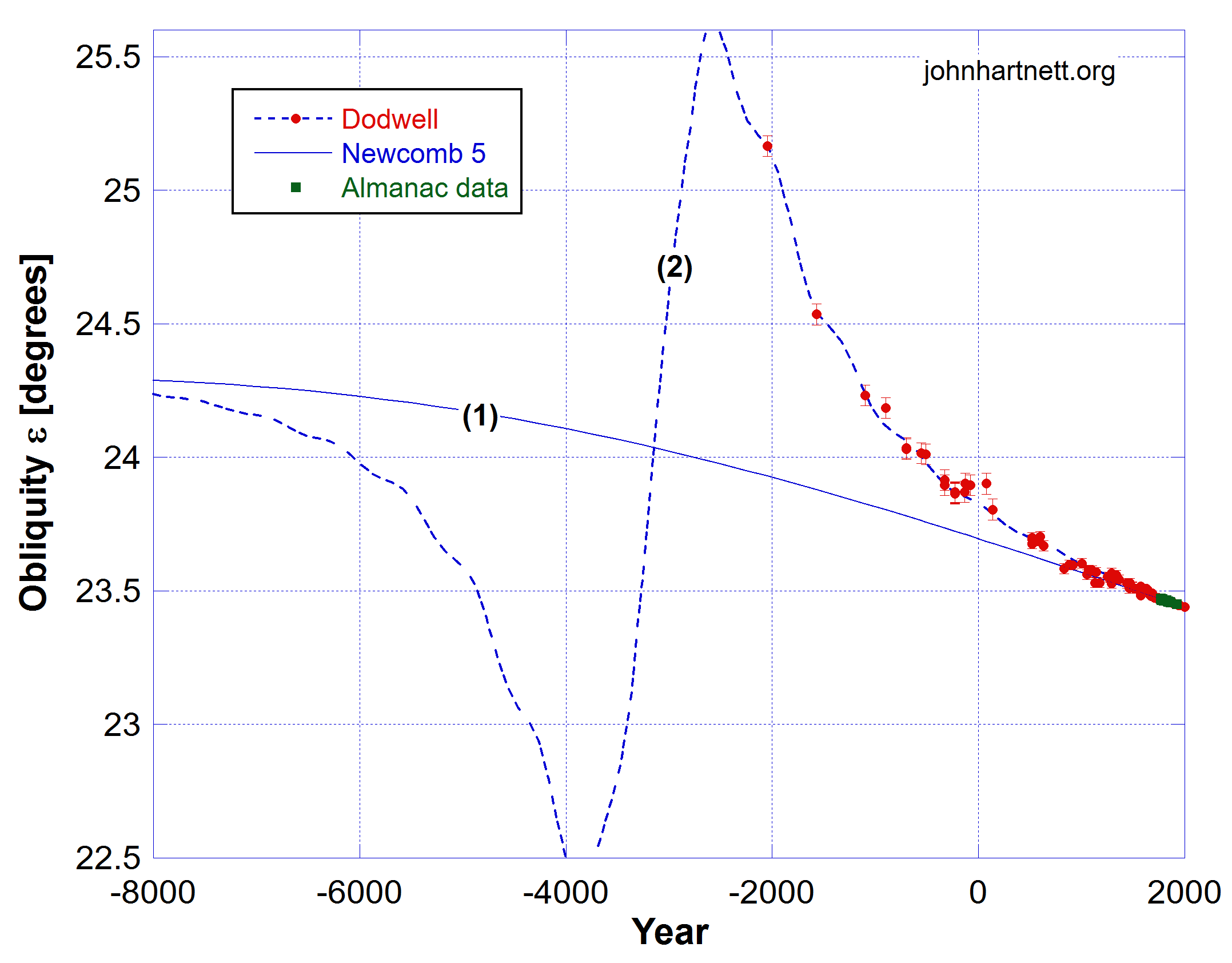
Considering the potential source of the Earth’s anomalous change in obliquity being of astronomical origin then an oscillation on top of the changing trend seen in the Lorentzian line is conceivable.
Currently my favoured origin is in the change of tilt of the Earth’s core, which induced a change in the planet’s spin axis. An additional sinusoidal oscillation/perturbation is also conceivable from that source.
Here I investigate the effect of adding such a small oscillation to the Earth’s obliquity.
In addition I have added an extra 30 data points for obliquity from archival records of the Nautical Almanac and supplied to me by Frank Hubeny. Those are labelled Almanac data (green) in the Figs here.
The modified Model 3, now called Model 3.1, describes the obliquity ε(t) as,
ε(t) = Newcomb(T) + Lorentzian(t){1+Ksin(t/t0+C)}, …. (1)
where t is years since the year 0, equal to BC/AD, and T is in centuries. Newcomb’s 5th order polynomial and my Model 3 Lorentzian is found in eqs (1) and (4) here. I have added a small sine wave oscillation to the Lorentzian curve. The unknown constants K, t0 and C are determined by the best curve fit using regression fit analysis. The best fit result is shown in Figs 1 through 3. All other parameters are the same as those determined previously.
The period of oscillation t0 = 105.1 ± 2.1 years. Coincidentally there is a 105 year oscillation in sunspot number, which could be related to gravitational influences on the Earth’s spin axis. The amplitude of the oscillation K = 0.00117° ± 0.00027°. Interestingly the current radius of nutation is 9.63 arcsec = 0.002675° as of April 10, 2025 (Gregorian). See Fig. 7 in my earlier report here. That means this oscillation is half that of nutation. The parameter C is a just phase term and doesn’t tell us much.
An initial inspection of Fig. 1 shows the earliest data have better fits to the new Model 3.1, which has the addition of a small sinusoidal oscillation.
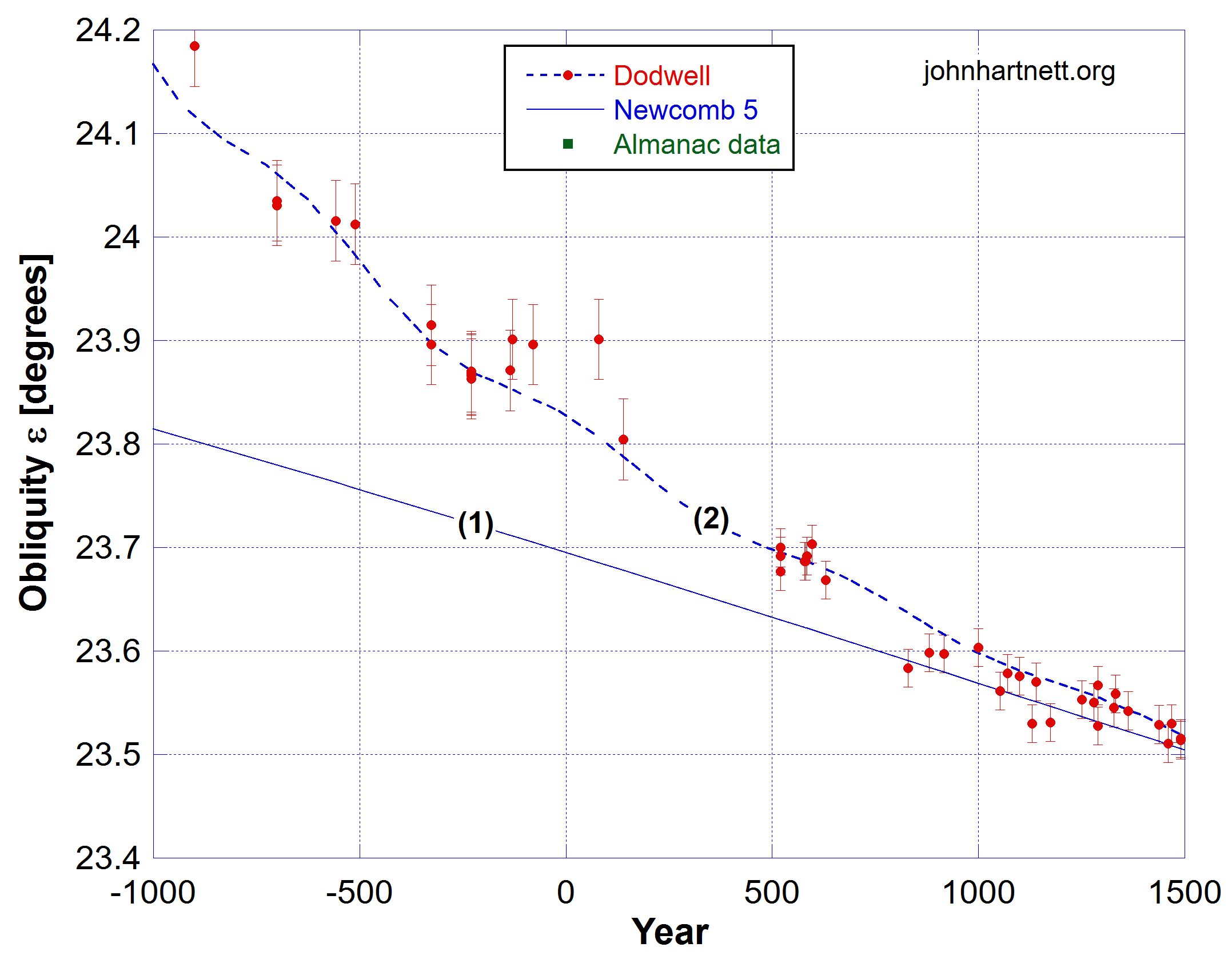
From Fig. 2 it is clear to see that a sinusoidal oscillation with a period of 105.1 ± 2.1 years is plausible. Fig. 3 shows the detail for the last 400 years.
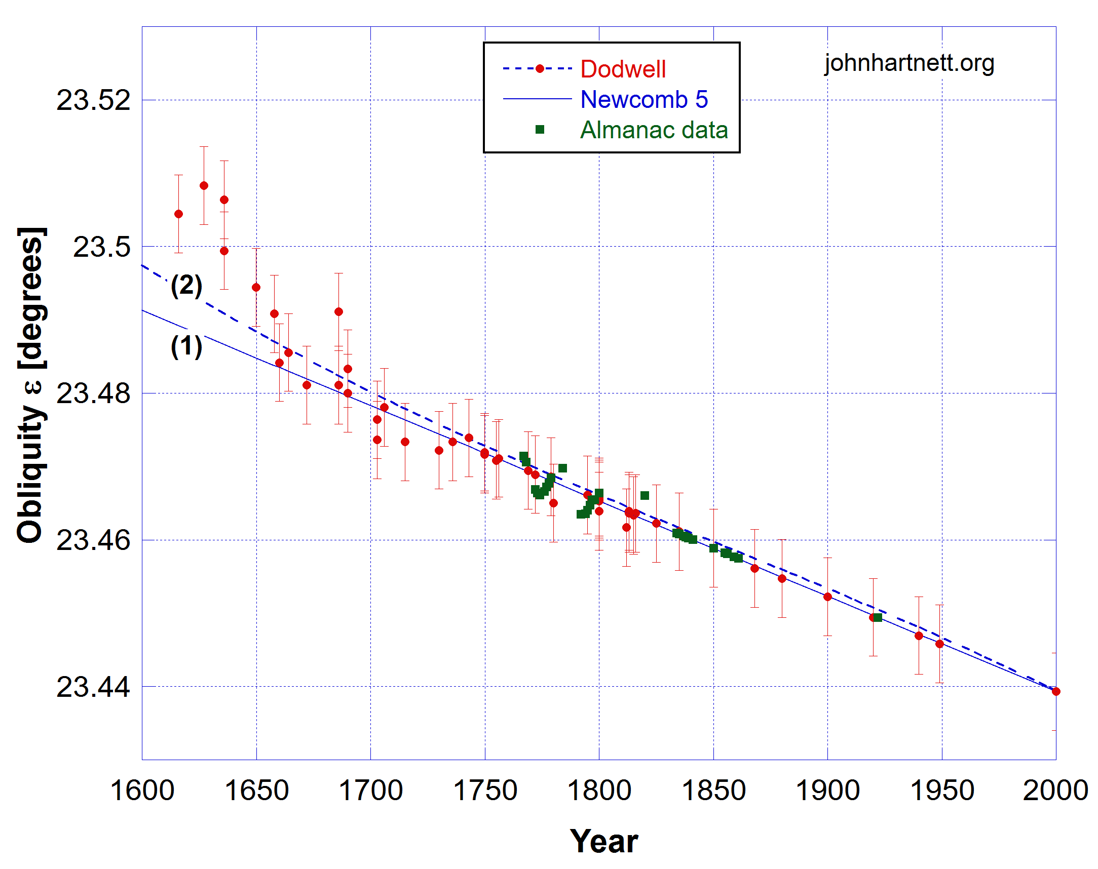
Here I have plotted, with green squares, the extra 30 data from the Nautical Almanac, which lay within the error bars of Dodwell’s data. For clarity I have not added error bars to the N. Almanac data (green squares).
It is obvious that some oscillation is seen in those (green) Nautical Almanac data though not with a period of 105 years.
The application of a sinusoidal oscillation raises the expected obliquity over this period but the modelled dashed curve lies well within the 1σ errors of Dodwell’s data over this time period.
Previously I mentioned that one concern I had was the systematic trend in the residuals when applying either Model 1 or Model 3 for the obliquity. In Figs 4 and 5 I take a fresh look at the residuals when my Model 3.1 is applied.
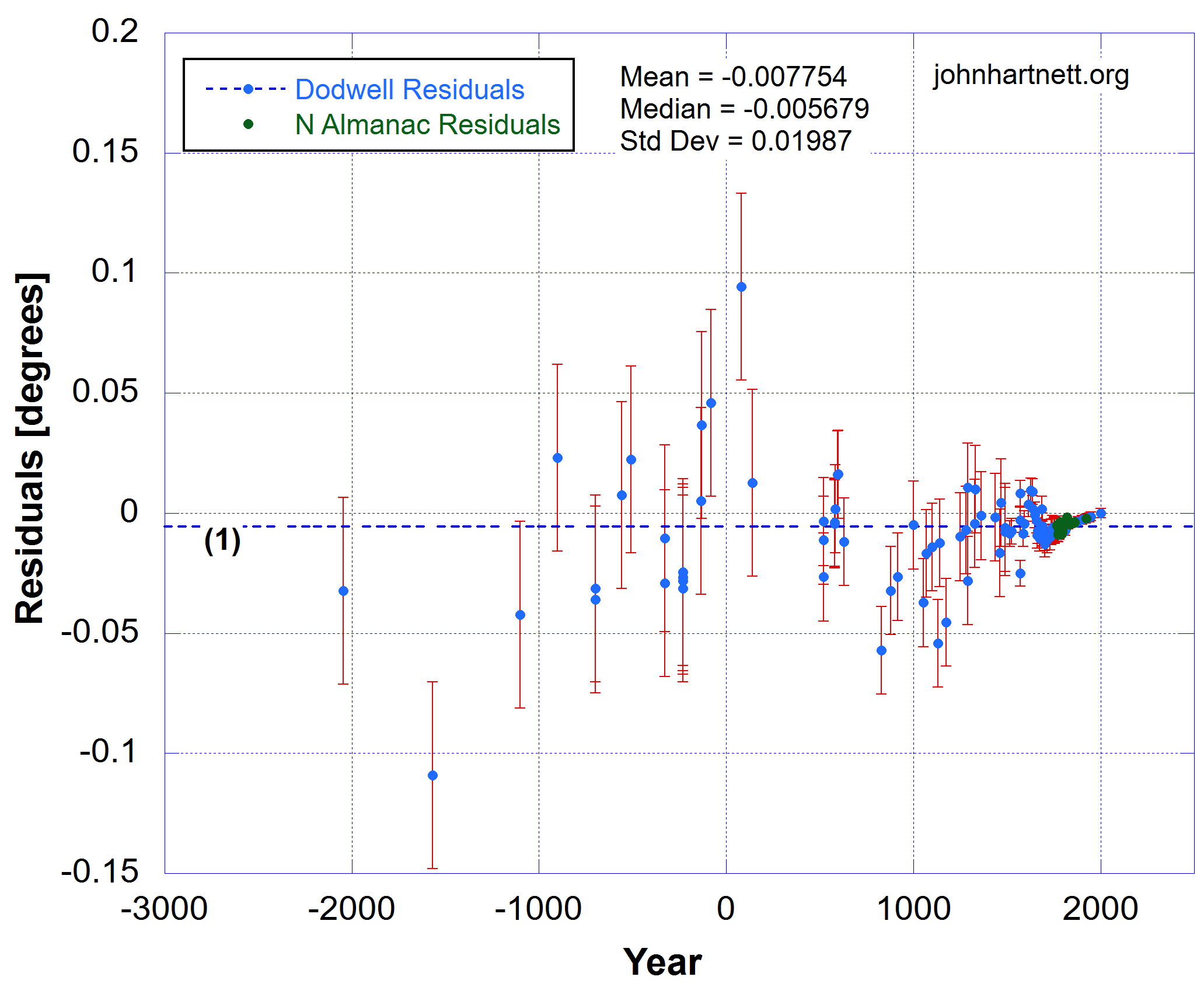
Actually there is a slight improvement in residuals for the earliest data and though the data appear to be well distributed around zero, the median is 10x larger than without the added sinusoidal oscillation. The trend is still seen in the residuals and the Nautical Almanac data are also consistent with that. See Fig. 5.
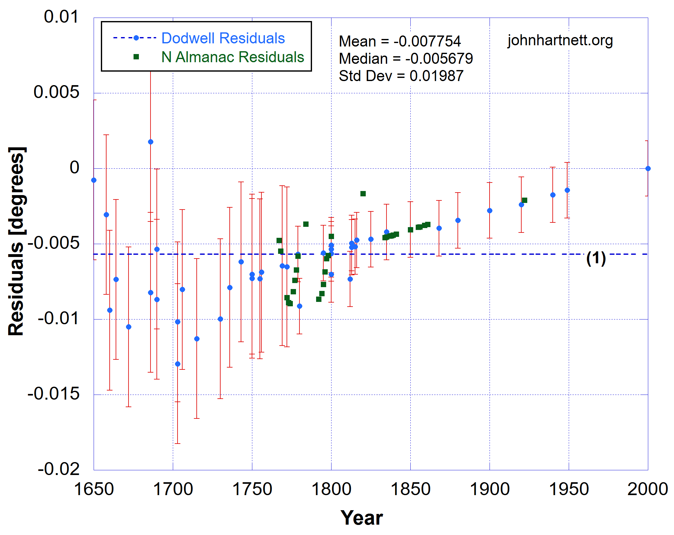
The Nautical Almanac data (green) nearly all lie within the 1σ errors on the residuals. Though the median of the residuals here with Model 3.1 is 10x larger than that using Model 3, the trend in the residuals tends to zero in the year 2000 AD.
In summary, the added Nautical Almanac data do not add anything new to the analysis but are consistent with previous Dodwell data. A small sinusoidal oscillation in the obliquity, smaller in amplitude than the known nutation of the planet currently, could explain some deviations from the expected Lorentzian line shape. Perhaps it is worth exploring a damped (decaying) sinusoidal oscillation. That might better fit to earlier excursions from the Lorentzian line. And if the Lorentzian perturbation turned off in the year 1800 AD all measured obliquity data would agree with the Newcomb polynomial formula.
Required Reading
- Obliquity of Earth’s Axis | How Has It Changed?
- Can We Know the Year of Noah’s Flood?
- Evidence of Creation | Mechanism Causing Perturbation in Obliquity of Planet Earth
Recommended Viewing
The Amazing Science of Young Earth Creation (2 hour video explaining a lot of this)
Free Subscribers
Subscribe to our Newsletters as a Free Subscriber and be notified by email. Just put your email address in the box at the bottom of your screen.
You’ll get an email each time we publish a new article. It is quick and easy to do and totally free. You only need do it once.
Premium Subscribers
Subscribe to our Newsletters as a Premium Subscribers at $5 USD/month or $30 USD/year (you choose).
Paid Premium Subscribers will get exclusive access to certain content I publish. That will only cost you a cup of coffee per month.
Also you’ll be able to download, for free, a PDF of my book Apocalypse Now and also a PDF of my book Physics of Creation The Creator’s Ultimate Design for Earth.
You can download them from the link below.
This is how you can support my work. I have been publishing this website for 10 years now and up to 2024 I never asked for any support.
Press the button “Premium” on the front page to find a list of Premium content. Thanks so much to all supporters.
At a minimum, please join as a Free Subscriber. It’ll cost you nothing. It may also help me beat the shadow banning of some posts.


Leave a comment