Bible Science Forum

On the fourth day God created the Sun and the Moon and by inference the rest of the solar system. He had already created Earth on the first day. Then the biblical text (Genesis 1: 16) reports “He made the stars also”.

On a moonless night the heaven displays a myriad of stars visible to the naked eye but billions upon billions more may be seen with the aid of modern large telescopes. It is estimated that the visible Universe  contains a hundred billion galaxies each containing on average a hundred billion stars. That is 10²² stars which may be written out this way as 10,000,000,000,000,000,000,000 stars. And the Creator knows them all by name.

He tells the number of the stars; he calls them all by their names. Psalms  147:4

The word ‘tell’ used in this verse is translated from the Hebrew word  מָנָה manah, which has the meanings of not only to enumerate but also to appoint and prepare.  The Creator knows them all by name and He appointed them for His own glory (Ps 19:1). The fact that He knows them all by name implies a finite number. Indeed it is true 10²² is a lot of stars, but God is a very great God. He has placed our home the planet Earth in the solar system in a safe place in the Galaxy we call the Milky Way.

If the number of stars in finite, though very large, then is there an edge to that number? The stars are in galaxies and as we look out beyond our galaxy we see more galaxies.  So if there is only a finite number they must eventually come to an end? And is our location in space near the centre of all those galaxies?

Modern big bang cosmology teaches otherwise. It teaches that there is no centre and no edge. Either the Universe goes on forever, hence is infinite in extension, or, it is closed in on itself like the surface of a balloon. That means it is finite, but with no boundary. If you were to travel in space, hypothetically, for hundreds of billions of years at the speed of light you would never come to an edge. There is no outside of those galaxies. See THE UNIVERSE: FINITE OR INFINITE, BOUNDED OR UNBOUNDED. But the biblical text suggests otherwise. Certainly we can say that on Earth we are at the centre of God’s attention. But are we, or I should say, is our galaxy somewhere near the centre of the visible Universe? (The following has been edited from an article first published in Journal of Creation  24(2):105-107, 2010)

What do we observe in the Universe?

Do we see a uniform, or homogeneous, distribution of matter in the Universe? This is a very difficult question to answer, because the usual method of measuring the distances to large collections of very distant galaxies relies on the Hubble Law.

The Hubble law was a discovery of Edwin Hubble who related the redshift of the spectral lines in the light coming from nearby galaxies to the galaxy’s distance from Earth. The greater the distance the greater the redshift. Assuming that this inference is correct for the moment, the Hubble law is a method of determining distance to those galaxies.  But the exact form of the Hubble Law at high redshift (i.e. large distances) depends heavily on the particular details of any assumed cosmological model.

Nevertheless there have been a few large-scale mapping projects that take a slice of the heavens, measure the redshifts of the galaxies in view and plot their positions and inferred distances on a map, which we may see projected onto a plane.

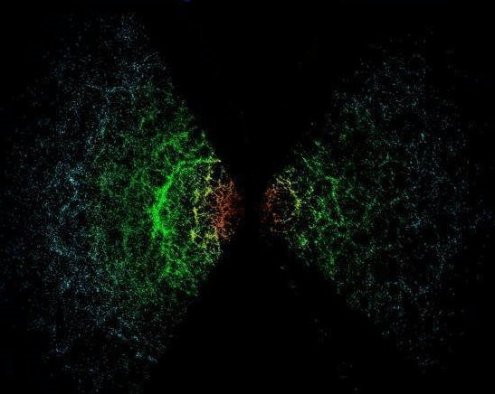
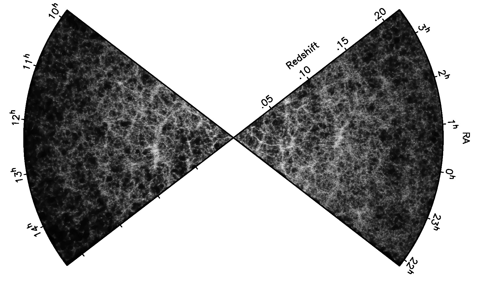
The 2dF Galaxy Redshift Survey (2dFGRS),¹ a joint UK–Australian project, sampled about two hundred thousand galaxies in 2-degree slices above and below the plane of the Galaxy. Fig. 1 shows a map of the measured galaxies as a function of distance from the apex, which represents the observer on Earth.

Another, the Sloan Digital Sky Survey (SDSS),² in 2003 announced the first measurements of galactic structures more than a billion light-years across and mapped about two hundred thousand galaxies in 6% of the sky. Later this was extended to more than one million galaxies.  A portion of these galaxies is shown projected onto a plane, in fig. 2.

It would appear from these maps that the assumption of homogeneity, the idea that the galaxies are smoothly and uniformly distributed throughout the Universe, cannot be supported. Figs 1 and 2 show not only concentric but also circular structures centred near our galaxy more clearly than do earlier maps. We see what is called ‘cosmic web’ , a series of voids and connected filaments, but also we see a general concentric structure of galaxies, which tend to lie on circles spaced equidistant from the centre.  This is particularly obvious to the human eye in the left hand side of Fig. 2.

This result is more than an artefact of the sampling technique because the density distribution of galaxies is expected to increase with distance in a big bang universe, as one looks back in time, until an expected decrease in number is observed due to the fact that the galaxies get too dim to be seen.

In these maps, the galaxy density seems to oscillate (decrease and increase periodically) with distance, hence the circular structures. This spatial galaxy density variation can result from the fact that galaxies are preferentially found at certain discrete distances.

Detailed analysis

Now it gets technical.

In a paper published in 2008,³ with a colleague, I showed that from Fourier analysis of galaxy number counts N(z) calculated for both SDSS and 2dF GRS, that galaxies have preferred periodic redshifts. Though many do not have any preferential redshift there is a small bias towards those that do.

We took all the galaxies in the survey and binned them or added up how many there were at a given redshift (z) and calculated the abundance of galaxies N(z) at each redshift. This is called a histogram. Such a histogram of redshift abundances for the SDSS data is shown by the black solid line in Fig 3.

The red dot-dash line represents the survey function. This is what we’d expect to get for a smooth uniform distribution of galaxies. Quite obviously this is not the case and the variation away from the survey function line indicates variations in the density of galaxies at the relevant redshift (z).

Then using a Discrete Fourier Transform (DFT) applied to those histograms N(z), we looked for periodic structure. For the non-mathematical or non-engineering oriented reader this is a technique when applied properly can detect periodic structure in even what may look to the eye like noise.

Data for 427,513 galaxies from the SDSS Fifth Data Release (DR5) were obtained where the data are primarily sampled from within about -10 to 70 degrees Declination (DEC) from the celestial equator. Also, data for 21,414 galaxies were obtained from the 2dF GRS where the data are confined to within 2 degrees DEC balanced between the Northern and Southern hemispheres. Those coordinates tell you the position on the sky, which is largely determined by the directions of the unimpeded view of the night sky away from the disk of our galaxy.

Our DFT analysis found significant periodic redshift spacings of Δz = 0.0102, 0.0246, and 0.0448 in the SDSS data, with significance at a level of at least 4σ (4 standard deviations) and strong agreement with the same analysis from 2dF GRS data.

What does a 4σ (sigma) detection mean? It means, if it is real, it has a 99.994% probability of being correct.

In the sciences generally the higher sigma the better. Most require 5 sigmas (or a probability of 99.99994%) as the threshold for a discovery, but some discoveries have been made at the level of 3 sigmas or less.⁴ See Fig. 4.

The Cryogenic Dark Matter Search collaborators claimed some bumps in their data might be a weakly interacting massive particle (WIMP) signal at the 3-sigma level.  But it was not a detection. And a faster-than-light neutrinos claim was wrong even though it was from a 6-sigma result.

Our results then tells us we need to do more investigation.  This is only preliminary. That research is underway with the help of the Institute of Creation Research (ICR) and we are hoping to report more on that later.  But now that we have a feel for the significance of this, let’s continue.

Real-space or redshift-space structure?

If one then applies the Hubble Law,⁵ that is, one assumes that the Hubble Law applies to these relatively low-redshift galaxies (z < 0.35) without assuming any cosmology, then the conclusion one gets is that the galaxies preferentially tend to be located on concentric shells with periodic real-space intervals Δr. These were determined from,

by replacing redshift z with redshift intervals Δz, resulting in regular real-space radial distance intervals Δr. And by combining the results from both surveys, we get

Δr = 31.7 ±1.8 h^-1 Mpc,  73.4 ± 5.8 h^-1 Mpc  and 127 ± 21 h^-1 Mpc,

where the Hubble constant H₀ = 100 km/s/Mpc and the parameter h = H₀/100, as used in standard cosmology. The parameter c is the speed of light in vacuum. Using a commonly used value for h = 0.7 from a Hubble constant value of 70 km/s/Mpc one can convert these interval into distance spacing in units of millions of parsecs.

In the usual analysis, in standard cosmology, the spatial two-point correlation function is used to define the excess probability, compared to that expected for a random distribution, of finding a pair of galaxies at a given separation. This involves the assumption of the Cosmological Principle.⁶ This is then under the assumption that there is no special place, no centre and all points in the Universe are equivalent. As a result, the power spectrum P(k) is derived from the two-point correlation function.⁷ The power spectrum is predicted by theories for the formation of large-scale structure in the universe and compared with that measured, or, more precisely, calculated from the available data.

The power spectrum P(k) is used to look for mass density fluctuations on various scales over cosmological time. There it is assumed that looking back in redshift space is looking back over cosmological time and, in the light of the Cosmological Principle, any density fluctuations are simply evidence of the scale of clustering at some past epoch (z), since there is no special or preferred frame to view the universe from. In deriving P(k), a windowing function (usually a Gaussian) is applied to reduce the noise seen in the density fluctuations as a function of k or 1/Δz.  This is to reduce artefacts  in the resulting P(k), that result from the edges of finite data sets. (k is a sort of spatial frequency; more correctly a phase space.) Care must be taken, as applying a windowing function may have the effect of smoothing out the ‘signal’ we are looking for contained in the ‘peaks’ at small-redshift intervals or high 1/Δz frequencies. We applied this method, without the Gaussian windowing function, and we still found significant redshift space (actually k-space) periodicity in both data sets at redshift intervals consistent with the first two listed above, i.e. at Δz = 0.0102 and 0.0246.

However a Discrete Fourier Transform (DFT) of the unsmoothed N(z) data is much more sensitive to finding redshift space periodicity at smaller values of Δz,  which means higher Fourier 1/Δz frequencies. And the third significant redshift periodicity, where Δr =127 ± 21 h^-1 Mpc, seen with the DFT method, is the same result discovered by Broadhurst et al. (1990)⁸ from a pencil-beam survey of field galaxies.

The latter is generally interpreted as the scale of galaxy clustering in the universe. This is referred to as the baryon acoustic oscillation (BAO) scale size in the standard model, with a scale size of Δr =110.4 ± 1.4 h^-1 Mpc.  The BAO scale is fixed by the sound horizon at the alleged decoupling epoch.⁹  It is supposed to be the distance that the expanding acoustic shells can travel in the big bang universe before decoupling. This value was determined from the study of the temperature anisotropies in the Cosmic Microwave Background (CMB). This is also measured in the  two-point correlation function analysis of the large galaxy survey data.

Also, we applied straight pair counting. Another way to determine if galaxies are separated by a periodic redshift interval is to build histograms by binning the number of pairs (N_pairs) of galaxies that have the same separation (Δz) in redshift space, then looking for over-abundance peaks in the N_pairs histograms. Since redshifts are measured radially from the observer at the centre of the distribution, this method detects redshift space separation with respect to that symmetry. As it turned out, it was not so sensitive but did still detect the first two listed above, i.e. at Δz = 0.0102 and 0.0246

Finally we did a correlation analysis between the two surveys. We compared N(z) from each by artificially shifting the redshift of the ith bin (determined between z_i − δz/2 and z_i + δz/2) in one survey and re-calculating the correlation function R² at each step. See ref. 3 for details. There is a significant spatial region of the 2dF GRS that has overlap with the SDSS and so we would expect R²  for the unshifted bins to show significant correlation. What we found was interesting. We found a periodicity in the R² correlation function with a period Δz ≈ 0.027. This is again the main visible-to-the-eye redshift periodicity.

Two ways to interpret the results

Now these results can be interpreted as either evidence for a real-space structure with our galaxy cosmologically near its centre, or as a redshift-space effect where the universe has undergone oscillations in its expansion rate over past epochs. The latter is what Hirano et al. (2008)¹⁰ advocated and we referred to it in ref. 3.

In Fig. 5, I have drawn a set of circles centred on the observer at Earth with a redshift interval of Δz = 0.0246. How do we interpret that evidence?

Either the effect is totally due to the expansion of the universe, and therefore only a redshift space effect, because redshift is one dimensional, or it results from real space structure. Since we are only able to sample the radial component of the redshift, assuming it results from the galaxies moving away from us, then it would only appear that the galaxies are arranged in rings (or shells in 3D space) due to the fact that in the past the universe’s rate of expansion oscillated, i.e its rate of expansion slowed then increased periodically. If this were the case then it should look like all galaxies are racing away from the centre and that these rings are centred exactly on the observer, never off-centre from the observer, not even by a small amount.¹¹

The subtlety here is that one is implicitly assuming that the distribution of galaxies in the universe must be essentially random on the very large scale with only the cosmic web of filaments and voids, an assumption from the Cosmological Principle. Hence anything else you see must be due to some effect other than real-space structure.

‘What really interests me is whether God had any choice in the creation of the world’—Albert Einstein¹²

However, if the effect is a real-space effect, it means that the galaxies are physically situated in concentric shells, which, in an expanding universe, are moving away from us at the centre. This interpretation also suggests that, at a minimum, the local universe we see around us has a special place, a centre, and we are there,or nearby. This idea is at odds with the Cosmological Principle, which, remember, has its origin in the notion that there is no Creator, no design and no purpose in the universe. Therefore, the idea that we may be living at or near the centre of the universe is abhorrent to all those who hold to atheistic and/or non-biblical worldviews.

It is not so easy to determine the real-space structure of the universe because we have no independent measure of distance in the universe. So when astronomers look at a map, they really are looking at a map of redshifts and directions in the sky from where the light has come. Then to get the radial distance to the source galaxy they have to assume the Hubble law.

However, there may be a way to distinguish between these two possibilities. As I mentioned, if the centre of the large-scale structure of galaxies around us coincides with our galaxy it would suggest that it is purely a redshift-space effect and not indicative of real space, though even that would still be impossible to prove because we have no independent measure of distance. But if the centre of concentric shells of galaxies coincides at some other point in space, away from where we are, then that indicates a real-space structure and not solely a redshift-space effect.

Real-space near galactocentric structure

In a second paper¹³ I found a real-space superstructure, possibly involving millions of galaxies, was favoured, with galaxies preferring to lie on periodically spaced concentric shells centred on a location about 26.86 h^-1 Mpc from here. Certainly, to date, this has not been ruled out. However, I made the assumption that for small redshifts it was valid to assume we are looking at spatial distribution of the galaxies in their redshifts.

Then I implemented an algorithm to artificially shift the centre in real space, recalculate what all the redshifts would be if observed from that new central point, re-determine N(z) and re-calculate the DFT from the new N(z). I then compared the magnitude of the second Fourier peak (for the dominant redshift space interval) to determine where the true physical centre should be. This is where the Fourier peak amplitude is maximized. I found that the centre of the concentric shells with Δz ≈ 0.0246 does not coincide with our galaxy’s position in space but that the centre is about 26.86 h^-1 Mpc or about 135 million light-years (assuming h = 0.7)  from here. That is still a relatively small distance on the very large scale of the structure analyzed—billions of light-years in extent.  So cosmologically speaking that places us near the centre of this giant cosmic structure.

Conclusion

The evidence is in favour of this effect being due to real-space structure because the spherical shells of periodic redshift are not centered on our galaxy. If it was a systematic effect due to observer bias, we would expect that the centre of the shells would coincide with the observer. Though this is still not conclusive, and more analysis is needed, we have evidence for a supermassive real-space structure, possibly involving millions of galaxies, with our Milky Way located somewhere near, but not actually at, its centre.

We are in a special place after all, definitely spiritually at the centre of God’s attention and also maybe physically somewhere near the centre of the largest galactic structure ever observed in the universe. We are here not by random chance but because God created the earth to be inhabited and He wanted to show us His glory.

‘For the invisible things of him from the creation of the world are clearly seen, being understood by the things that are made, even his eternal power and Godhead; so that they are without excuse’ (Romans 1:20).

And they are without excuse.

Update: 18/03/2019

Scientists at the Institute for Creation Research worked on trying to understand if there was any real significance to the idea of discrete galaxy redshifts which might imply galaxies arranged on concentric shells.  That research was never completed. They however have written a report on the work.  The results are inconclusive.

References

1. http://www.aao.gov.au/2df.
2. http://www.sdss.org.
3. Hartnett, J.G. and Hirano, K., Galaxy redshift abundance periodicity from Fourier analysis of number counts N(z) using SDSS and 2dF GRS galaxy surveys, Astrophysics and Space Science 318(1, 2):13–24, 2008; preprint available at: arxiv.org/abs/0711.4885.
4. A 2.5 Sigma Higgs Signal From The Tevatron!   http://www.science20.com/quantum_diaries_survivor/25_sigma_higgs_signal_tevatron-91654
5. Hubble Law: v = H₀ r, where v is the velocity of the expansion of the universe, as determined by the redshift of the galaxies in it. Here redshift z = v/c for small redshifts, where c is the speed of light in vacuum. The distance to the galaxy is represented by r, and H₀ is the Hubble constant, which has been very difficult to determine but nowadays lies somewhere between 65 and 75 km/s/Mpc.
6. It essentially assumes that the galaxies in the universe are uniformly yet randomly distributed throughout the cosmos on some very large scale. Therefore all observers at all locations in the universe at the same epoch should see the same distribution of galaxies. There are no favoured places. Richard Feynman succinctly describes the problem of the Cosmological Principle: “… I suspect that the assumption of uniformity of the universe reflects a prejudice born of a sequence of overthrows of geocentric ideas … It would be embarrassing to find, after stating that we live in an ordinary planet about an ordinary star in an ordinary galaxy, that our place in the universe is extraordinary … To avoid embarrassment we cling to the hypothesis of uniformity.” Feynman, R.P., Morinigo, F.B. and Wagner, W.G., Feynman lectures on gravitation, Penguin Books, London, p. 166, 1999.
7. The power spectrum is essentially the square of the Fourier frequencies in k-space but calculated with a windowing function. Here k =1/Δz is the inverse of the redshift interval.
8. Broadhurst, T.J., Ellis, R.S., Koo, D.C. and Szalay, A.S., Large-scale distribution of galaxies at the Galactic poles, Nature 343:726, 1990.
9. Komatsu, E. et al. 2009, Astrophysical Journal Suppl., 180, 330
10. Hirano, K., Kawabata, K. and Komiya, Z., Spatial periodicity of galaxy number counts, CMB anisotropy, and SNIa Hubble diagram based on the universe accompanied by a non-minimally coupled scalar field, Astrophys. Space Sci. 315:53, 2008.
11. This situation would also be indistinguishable from real space structure exactly centred on our galaxy.
12. Einstein made this remark to Ernst Straus, his assistant from about 1950–1953 at the Institute for Advanced Study at Princeton (Holton, G., Einstein’s third paradise, Daedalus, Fall 2003, pp. 26–34; p. 30, http://www.aip.org/history/einstein/essay-Einsteins-Third-Paradise.pdf, accessed 7 May 2010).
13. Hartnett, J.G., Fourier analysis of the large scale spatial distribution of galaxies in the universe; in: Proceedings of the 2nd Crisis in Cosmology Conference, Potter, F. (Ed.), Port Angeles, WA, ASP Conference Series 413:77–97, 2009.

 Additional resources

Read and watch:

• Book: Starlight Time and the New Physics
• DVD: Starlight Time and the New Physics